![Mechanical Properties]()
Mechanical Properties
Introduction to Mechanical Properties
Tensile property characterization of mild and High Strength Low Alloy steel (HSLA) traditionally was tested only in the rolling direction and included only yield strength, tensile strength, and total elongation. Properties vary as a function of orientation relative to the rolling (grain) direction, so testing in the longitudinal (0°), transverse (90°), and diagonal (45°) orientations relative to the rolling direction is done to obtain a better understanding of metal properties (Figure 1).
A more complete perspective of forming characteristics is obtained by also considering work hardening exponents (n-values) and anisotropy ratios (r-values), both of which are important to achieve improved and consistent formability.

Figure 1. Tensile Test Sample Orientation Relative to Rolling Direction
Hardness readings are sometimes included in this characterization, but hardness readings are of little use in assessing formability requirements for sheet steel. Hardness testing is best used to assess the heat treatment quality and durability of the tools used to roll, stamp, and cut sheet metal.
The formability limits of different grades of conventional mild and HSLA steels were learned by correlating press performance with as-received mechanical properties. This information can be fed into computer forming simulation packages to run tryouts and troubleshooting in a virtual environment. Many important parameters can be measured in a tensile test, where the output is a stress-strain curve (Figure 2).

Figure 2: Representative Stress-Strain Curve Showing Some Mechanical Properties
Press shop behavior of Advanced High-Strength Steels is more complex. AHSS properties are modified by changing chemistry, annealing temperature, amount of deformation, time, and even deformation path. With new microstructures, these steels become “Designer Steels” with properties tailored not only for initial forming of the stamping but in-service performance requirements for crash resistance, energy absorption, fatigue life, and other needs. An extended list of properties beyond a conventional tensile test is now needed to evaluate total performance with virtual forming prior to cutting the first die, to ensure ordering and receipt of the correct steel, and to enable successful troubleshooting if problems occur.
With increasing use of advanced steels for value-added applications, combined with the natural flow of more manufacturing occurring down the supply chain, it is critical that all levels of suppliers and users understand both how to measure the parameters and how they affect the forming process.
Highlights
-
- The multiphase microstructure in Advanced High Strength Steels results in properties that change as the steel is deformed. An in-depth understanding of formability properties is necessary for proper application of these steels.
- Tensile test data characterizes the ability of a steel grade to perform with respect to global (tensile and necking) formability. Different tests like hole expansion and bending characterize performance at cut edges or bend radii.
- DP steels have higher n-values in the initial stages of deformation compared to conventional HSLA grades. These higher n-values help distribute deformation more uniformly in the presence of a stress gradient and thereby help minimize strain localization that would otherwise reduce the local thickness of the formed part.
- The n-value of certain AHSS grades, including dual phase steels, is not constant: there is a higher n-value at lower strains followed by a drop as strain increases.
- TRIP steels have a smaller initial increase in n-value than DP steels during forming but sustain the increase throughout the entire deformation process. Part designers can use these steels to achieve more complex geometries or further reduce part thickness for weight savings.
- TRIP steels have retained austenite after forming that transforms into martensite during a crash event, enabling improved crash performance.
- Normal anisotropy values (rm) approximately equal to 1 are a characteristic of all hot-rolled steels and most cold-rolled and coated AHSS and conventional HSLA steels.
- AHSS work hardens with increasing strain rate, but the effect is less than observed with mild steel. The n-value changes very little over a 105 (100,000x) increase in strain rate.
- As-received AHSS does not age-harden in storage.
- DP and TRIP steels have substantial increase in YS due to a bake hardening effect, while conventional HSLA steels have almost none.
![Mechanical Properties]()
2ndGen AHSS, AHSS, Steel Grades
TWinning Induced Plasticity (TWIP) steels have the highest strength-ductility combination of any steel used in automotive applications, with tensile strength typically exceeding 1000 MPa and elongation typically greater than 50%.
TWIP steels are alloyed with 12% to 30% manganese that causes the steel to be fully austenitic even at room temperature. Other common alloying additions include up to 3% silicon, up to 3% aluminum, and up to 1% carbon. Secondary alloying additions include chromium, copper, nitrogen, niobium, titanium, and/or vanadium.D-29 The high alloying levels and substantially greater levels of strength and ductility place these into the 2nd Generation of Advanced High Strength Steels. Furthermore, due to the density of the major alloying additions relative to iron, TWIP steels have a density which is about 5% lower than most other steels.
Calling this type of steel TWIP originates from the characteristic deformation mode known as twinning. Deformation twins produced during sheet forming leads to microstructural refinement and high values of the instantaneous hardening rate (n-value). The resultant twin boundaries act like grain boundaries and strengthen the steel. On either side of a twin boundary, atoms are located in mirror image positions as indicated in the schematic microstructure shown in Figure 1. Figure 2 highlights the microstructure of TWIP steel after annealing and after deformation.

Figure 1: Schematic of TWIP steel microstructure.

Figure 2: TWIP steel in the annealed condition (left) and after deformation (right) showing deformation twins. The number of deformation twins increases with increasing strain.K-42
EDDS or Interstitial-Free or Ultra-Low Carbon steels are different descriptions for the most formable lower-strength steel. Possible test results for this grade are 150 MPa yield strength, 300 MPa tensile strength, 22% to 25% uniform elongation, and 45% to 50% total elongation. In contrast, test results on TWIP steels may show 500 MPa yield strength, 1000 MPa tensile strength, 55% uniform elongation, and 60% total elongation.
The stress-strain curves for these two grades are compared in Figure 3. The TWIP curves show the manifestation of Dynamic Strain Aging (DSA), also known as the PLC effect, with more details to follow.

Figure 3: Uniaxial tensile stress-strain curves for an interstitial-free (IF) extra-deep-drawing steel and an austenitic Fe-18%Mn-0.6%C-1.5%Al TWIP steel. Curves are presented both terms of engineering (s,e) and true (σ,ε) stresses and strains, respectively.D-30
Figure 4 compares the results of bulge testing ferritic interstitial-free (IF) steel and austenitic Fe-18%Mn-0.6%C-1.5%Al TWIP steel. The TWIP steel is still undamaged at a dome height that is 31% larger than the IF steel dome height at failure.D-30

Figure 4: Comparison of dome testing between EDDS and TWIP.D-30
Excellent stretch formability is associated with high n-values. Shown in Figure 5 is a plot showing how the instantaneous n-value changes with applied strain. N-value increases to a value of 0.45 at an approximate true (logarithmic) strain of 0.2 and then remains relatively constant until an approximate true strain of 0.3 before increasing again. The high and uniform n-value delays necking and minimizes strain peaks. Twins continue to form at higher strains, leading to finer microstructural features and continued increases in n-value at higher strains.

Figure 5: Instantaneous n-value changes with applied strain. TWIP steels have high and uniform n-value leading to excellent stretch formability.C-30
A microstructural deformation phenomenon known as the Portevin-LeChatelier (PLC) effect occurs when deforming some TWIP steels to higher strain levels. The PLC effect is known by several other names as well, including jerky flow, discontinuous yielding, and dynamic strain aging (DSA).
The severity varies with alloy, strain rate, and deformation temperature. Figure 6 shows how DSA affects the appearance of the stress strain curve of two TWIP alloys.D-29 The primary difference in the alloy design is the curves on the right are for steel containing 1.5% aluminum, with the curves on the left for a steel without aluminum. The addition of aluminum delays the serrated flow until higher levels of strain. Note that both alloys have negative strain rate sensitivity.

Figure 6: Influence of aluminum additions on serrated flow in Fe-18%Mn-0.6%C TWIP (Al-free on the left) and Fe-18%Mn-0.6%C-1.5% Al TWIP (Al-added on the right).D-29
The primary macroscopic manifestations of the Portevin-LeChatelier (PLC) effect areD-29:
- negative strain rate sensitivity.
- stress-strain curve showing serrated or jerky flow, indicating non-uniform deformation. Strain localization takes place in propagating or static deformation bands.
- the strain rate within a localized band is typically one order of magnitude larger, while that outside the band is one order of magnitude lower, than the applied strain rate.
- limited post-uniform elongation, meaning uniform elongation is just below total elongation. Said another way, fracture occurs soon after necking initiation.
The PLC effect leads to relatively poor sheared edge expansion, as measured in a hole expansion test. Figure 7 on the left highlights the crack initiation site in a sample of highly formable EDDS-IF steel, showing the classic necking appearance with extensive thinning prior to fracture. In contrast, note the absence of necking in the TWIP steel shown in the right image in Figure 7.D-29
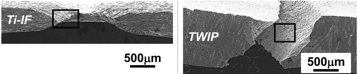
Figure 7: Sheared edge ductility comparison between IF (left) and TWIP (right) steel. TWIP steels lack the sheared edge expansion capability of IF steels.D-29
The stress-strain curves of several TWIP grades are compared in Figure 8.

Figure 8: Engineering stress-strain curve for several TWIP Grades.P-18
Complex-shaped parts requiring energy absorption capability are among the candidates for TWIP steel application, Figure 9.

Figure 9: Potential TWIP Steel Applications.N-24
Early automotive applications included the bumper beam of the 2011 Fiat Nuova Panda (Figure 10), resulting in a 28% weight savings and 22% cost savingsN-24 over the prior model which used a combination of PHS and DP steels.D-31

Figure 10: Transitioning to a TWIP Bumper Beam Resulted in Weight and Cost Savings in the 2011 Fiat Nuova Panda. N-24, D-31
In the 2014 Jeep Renegade BU/520, a welded blank combination of 1.3 mm and 1.8 mm TWIP 450/950 (Figure 11) replaced a two-piece aluminum component, aiding front end stability while reducing weight in a vehicle marketed for off-road applications.D-31

Figure 11: A TWIP welded blank improved performance and lowered weight in the 2014 Jeep Renegade BU/520.D-31
Also in 2014, the Renault EOLAB concept car where the A-Pillar Lower and the Sill Side Outer were stamped from TWIP 980 steel.R-21 By 2014, GM Daewoo used TWIP grades for A-Pillar Lowers and Front Side Members, and Hyundai used TWIP steel in 16 underbody parts. Ssangyong and Renault Samsung Motors used TWIP for Rear Side Members.I-20
Other applications include shock absorber housings, floor cross-members, wheel disks and rims, wheelhouses, and door impact beams.
A consortium called TWIP4EU with members from steel producers, steel users, research centers, and simulation companies had the goal of developing a simulation framework to accurately model the complex deformation and forming behavior of TWIP steels. The targeted part prototype component was a backrest side member of a front seat, Figure 12. Results were published in 2015.H-58

Figure 12: TWIP4EU Prototype Component formed from TWIP Steel.H-58
In addition to a complex thermomechanical mill processing requirements and high alloying costs, producing TWIP grades is more complex than conventional grades. Contributing to the challenges of TWIP production is that steelmaking practices need to be adjusted to account for the types and amounts of alloying. For example, the typical ferromanganese grade used in the production of other grades has phosphorus levels detrimental to TWIP properties. In addition, high levels of manganese and aluminum may lead to forming MnO and Al2O3 oxides on the surface after annealing, which could influence zinc coating adhesion in a hot dip galvanizing line.D-29
Critical to the performance of TWIP steels is having a microstructure that is fully austenitic. This is achieved with relatively high carbon (C > 0.5%) and manganese (Mn > 15%). These levels put the alloy at risk for hydrogen embrittlement, otherwise known as hydrogen-induced delayed fracture. Additions of aluminum were found to be effective in improving the resistance to delayed fracture. However, the levels of aluminum needed substantially reduced the castability of the molten alloy during continuous casting due to the propensity for aluminum to oxidize, which results in nozzle blockage and slag entrapment.
To reduce the amount of Al and consequently improve the castability of TWIP steels without reducing their resistance to delayed fracture, rare earth (RE) elements can be used. Rare earth metals react with H2 and form metal hydrides that are much more stable than the ordinary types of hydrogen entrapments in steels.Z-19
During annealing, manganese diffuses to the surface and oxidizes. The enriched manganese at the surface produces an oxidized layer that reduces the zinc wettability on the steel surface, and limits the ability to achieve a continuous galvanized coating. Solely using a high dew point atmosphere, such as the production strategy with QP steels, is insufficient in these high-Mn TWIP alloys.
A surface treatment process of annealing in a +10°C dew point to promote internal oxidation rather than external oxidation, combined with a subsequent pickling operation to remove any surface manganese oxides, results in a fully austenitic substrate covered by a lean-Mn decarburized ferrite layer, Figure 13. This strategy has led to the commercialization of hot-dip galvanized TWIP steels.P-32

Figure 13: Cross sectional microstructure of TWIP steel after targeted processing to improve galvanizability.P-32
Blog, main-blog
A New Software Application for Thin Wall Section Analysis
Advanced High-Strength Steel (AHSS) grades offer increased performance in yield and tensile strength. However, to fully utilize this increased strength, automotive beam sections must be designed carefully to avoid buckling of the plate elements in the section. A new software application, Geometric Analysis of Sections—GAS2.0, available through the American Iron and Steel Institute, is a tool to aid in this design effort.
Plate Buckling in Automotive Sections
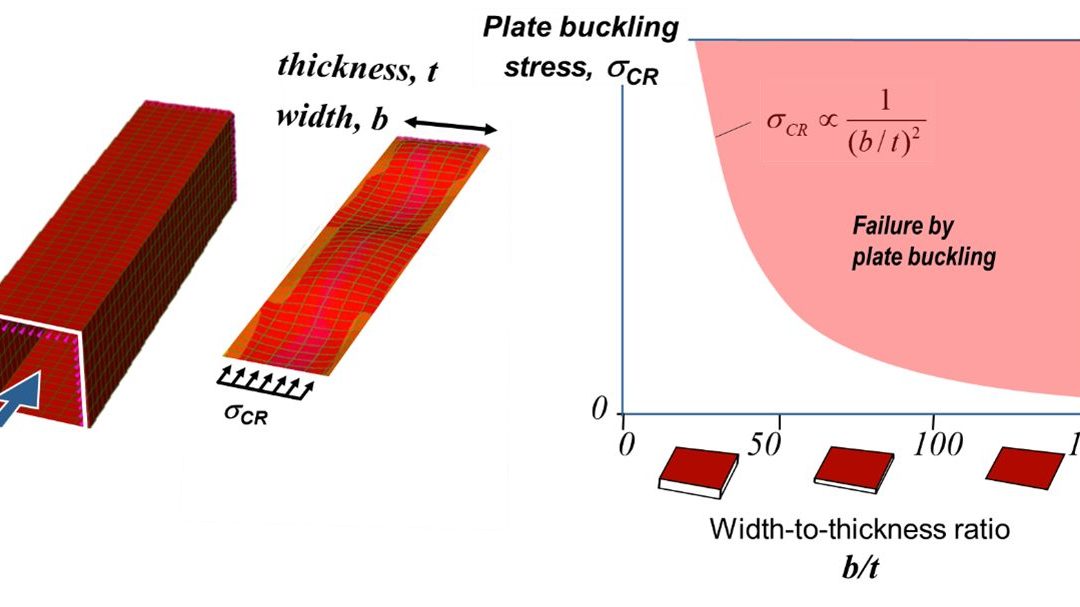
To understand how plate buckling affects the strength of a thin walled beam consider Figure 1. A square beam is made of four identical plates connected at their edges. Under an axial compressive load each plate may buckle. Considering just one of the plates, the stress that will cause buckling depends on the ratio of plate width and thickness (b/t). Thinner wider plates with large b/t ratio will buckle at a lower stress than thicker narrower plates.
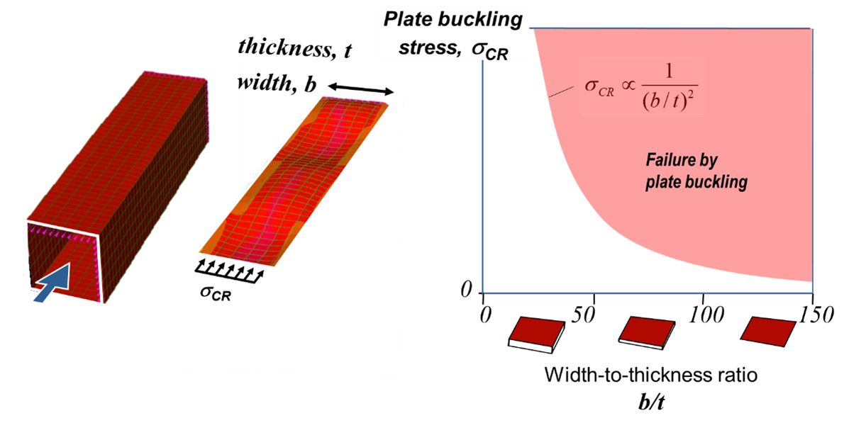
Figure 1: Plate Buckling Behavior.
Now consider a plate of mild steel (200 MPa yield stress) which has been designed to buckle just as yield stress is reached, Point A in Figure 2. The plate would have a b/t ratio of approximately 60. This design is taking full advantage of the yield strength of the material.
Now consider the same plate but substituting an AHSS grade (600 MPa yield stress) as shown in Figure 2. The plate will buckle at the same 200 MPa before reaching the material’s potential, Point B in the figure. To take advantage of this materials yield strength, the proportions of the plate will need to be changed, Point C. This illustration demonstrates the need to consider plate buckling particularly in the application of AHSS grades.
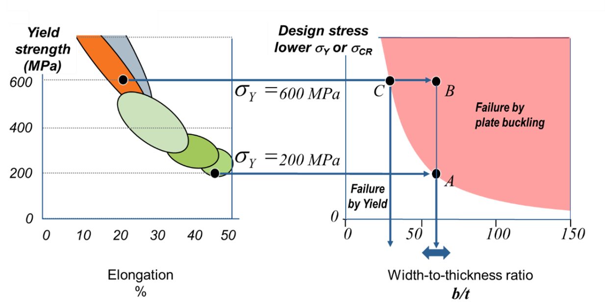
Figure 2: AHSS Substitution in a Plate.
Moving from a single plate to the more complex case of a beam section of several plates, consider Figure 3. On the left is the beam made of four plates with a compressive load causing the plates to just begin to buckle. However, this condition does not represent the maximum load carrying ability of the beam. The load can be increased until the stress at the corners of the buckled plates are at the material yield stress, center in Figure 3. Note that in this condition the stress distribution across the plate is nonlinear with lower stress in the center of each plate. One means to model this complex state is by using an imaginary Effective Section. Here the center portion is visualized as being removed and the remainder of the section is stressed uniformly at yield. The amount of plate width to be removed is determined by theory.W-21, A-42, Y-9, M-18 The effective section is a convenient way to visualize the efficiency of a section design given the material grade and provides an estimate of the maximum load carrying ability of the beam.
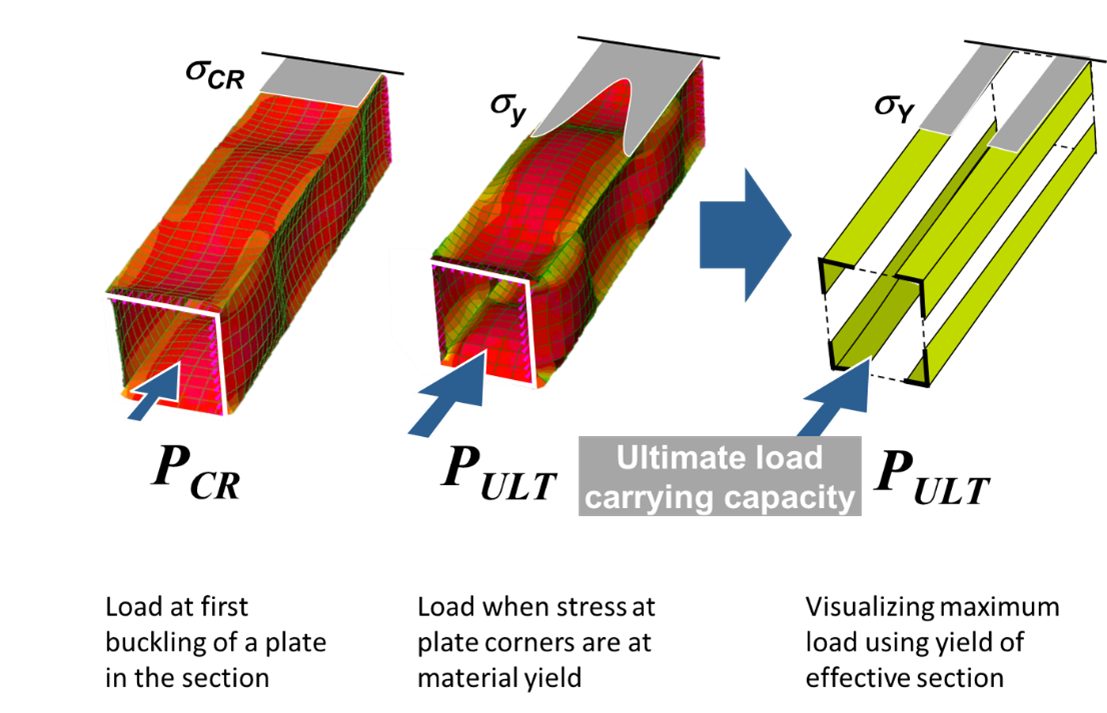
Figure 3: Concept of Effective Section.
Geometric Analysis of Sections – GAS2.0
Geometrical Analysis of Sections software determines the effective section for complex automotive sections. Figure 4 illustrates the GAS2.0 user interface. The user has the ability to construct sections or to import section data from a CAD system. Material properties for 63 steel grades are preloaded with the ability to also add user-defined steel grades. Two types of analysis are available. Nominal analysis, which provides classical area properties of the section, and Effective analysis which determines the effective section at material yield. Figure 5 summarizes both the tabular results and graphical results for each type of analysis.
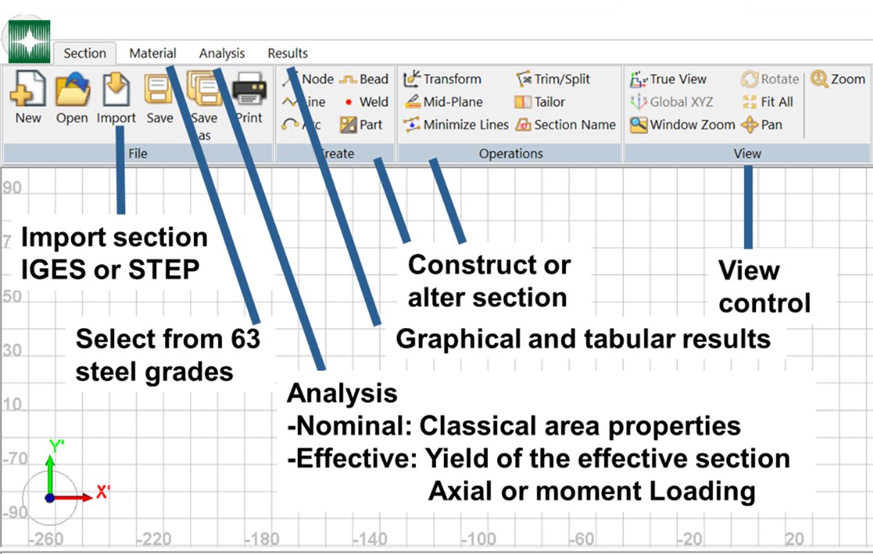
Figure 4: GAS2.0 User Interface.
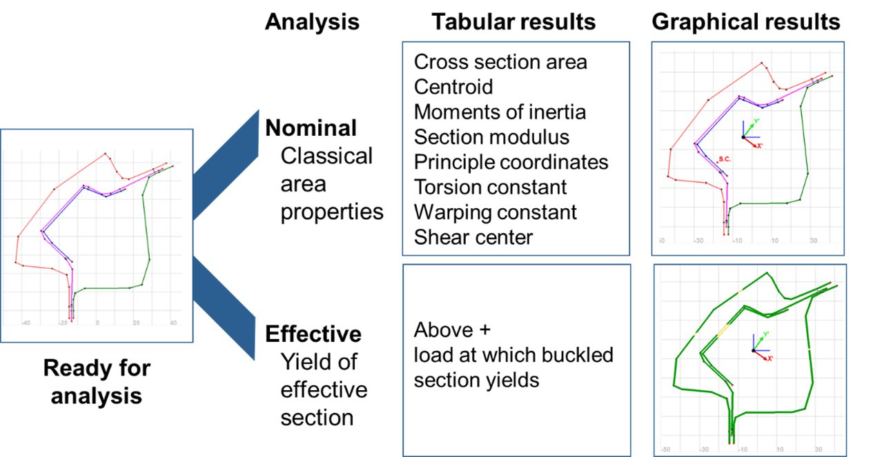
Figure 5. GAS2.0 Analysis Results.
Figure 6 illustrates an example of an Effective Analysis for a rocker section. In the graphical screen, the effective section is shown in green. Ideally, the whole section would be effective to fully use the materials yield capability. Also shown in the graphical screen are the section centroid, orientation of the principle coordinates, and stress distribution. In the right text box are tabular results. At the bottom of the tabular results is the axial load that causes this stress state and represents the ultimate load carrying ability of this section.
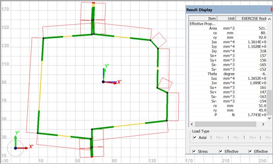
Figure 6: GAS2.0 Graphical Results.
It is clear that much of the material in the section of Figure 6 is not fully effective. GAS2.0 allows the user to conveniently modify the section. For example, in Figure 7 a bead has been added to the left side wall increasing its bulking resistance. Note that the side wall is now largely effective, and the ultimate load at the bottom of the text box has increased substantially.
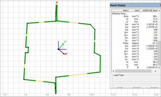
Figure 7: Improved Design Concept.
Role of GAS in the Design Process
GAS2.0 can play a significant role in early stage design, see Figure 8, by quickly creating initial designs which are more likely to function and to ensure that adequate package space is set aside for structure. This will result in fewer problems to fix later in the design sequence. During the detail design stage, GAS2.0 can supplement Finite Element Analysis by identifying problems earlier, and by screening design concepts for those with the greatest promise prior to more detailed analysis by FEA.
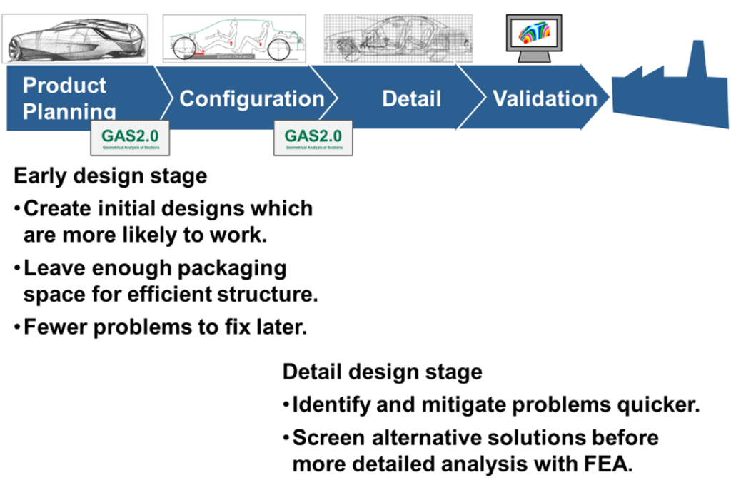
Figure 8: Role of GAS2.0 in Design Process.
GAS2.0 is available for free download at www.steel.org, Included in the resources at steel.org is an American Iron and Steel Institute introductory webinar conducted by Dr. Don Malen on 16 June 2020, as well as a number of GAS2.0 tutorials and training modules.
Resistance Spot Welding
Parameter Guidelines
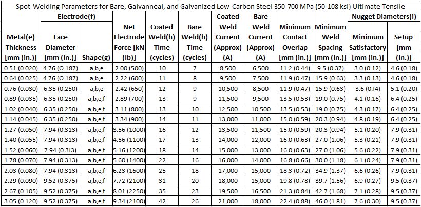
In summary, Tables 1 and 2 provide the AWS C1.1 Spot Welding Parameter Guidelines link to Recommended Practices for Resistance Welding. These general guidelines can be used to approximate which parameters can be used to begin the Resistance Spot Welding (RSW) process of a specific part thickness. From the recommended parameters, changes can be made on a specific stack-up to ensure an acceptable strength and nugget size for a particular application. Additionally, more complicated RSW parameter guidelines using a pulsation welding schedule with AC 60 Hz for welding AHSS is included in Table 3.
Table 1: Spot welding parameters for low-carbon steel 350-700 MPa (AHSS).A-14
- Use of coated parameters recommended with the presence of a coating at any faying surface.
- These recommendations are based on available weld schedules representing recommendations from resistance welding equipment suppliers and users.
- For intermediate thicknesses parameters may be interpolated.
- Minimum weld button shear strength determined as follows:
- ST = ((-8.83×10⁻⁷ × S2 + 1.34×10⁻³ × S + 1.514) × S × 4t1.5)/1000
- ST = Shear Tension Strength (kN)
- S = Base Metal Tensile Strength (MPa)
- t = Material Thickness (mm)
- Metal thicknesses represent the actual thickness of the sheets being welded. In the case of welding two sheets of different thicknesses, use the welding parameters for the thinner sheet.
- Welding parameters are applicable when using electrode materials included in RWMA Classes 1 , 2, and 20.
- Electrode shapes listed include: A-pointed, B-domed, E-truncated, F-radiused. Figure 2 shows these shapes.
- The use of Type-B geometry may require a reduction in current and may result in excessive indentation unless face is dressed to specified diameter.
- The use of Type F geometry may require an increase in current.
- Welding parameters are based on single-phase AC 60 Hz equipment.
- Nugget diameters are listed as:
- Minimum diameter that is recommended to be considered a satisfactory weld.
- Initial aim setup nugget diameter that is recommended in setting up a weld station to produce nuggets that consistently surpass the satisfactory weld nugget diameter for a given number of production welds.
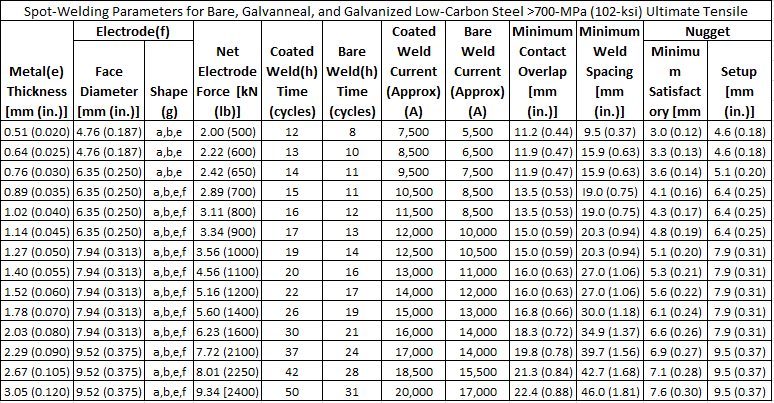
Table 2: Spot welding parameters for low-carbon steel >700 MPa (AHSS). A-14
- Use of coated parameters recommended with the presence of a coating at any faying surface.
- These recommendations are based on available weld schedules representing recommendations from resistance welding equipment suppliers and users.
- For intermediate thicknesses parameters may be interpolated.
- Minimum weld button shear strength determined as follows:
- ST = ((-8.83×10⁻⁷ × S2 + 1.34×10⁻³ × S + 1.514) × S × 4t1.5)/1000
- ST = Shear Tension Strength (kN)
- S = Base Metal Tensile Strength (MPa)
- t = Material Thickness (mm)
- Metal thicknesses represent the actual thickness of the sheets being welded. In the case of welding two sheets of different thicknesses, use the welding parameters for the thinner sheet.
- Welding parameters are applicable when using electrode materials included in RWMA Classes 1, 2, and 20.
- Electrode shapes listed include: A-pointed, B-domed, E-truncated, F-radiused. Figure 2 shows these shapes.
- The use of Type-B geometry may require a reduction in current and may result in excessive indentation unless face is dressed to specified diameter.
- The use of Type F geometry may require an increase in current.
- Welding parameters are based on single-phase AC 60 Hz equipment.
- Nugget diameters are listed as:
- Minimum diameter that is recommended to be considered a satisfactory weld.
- Initial aim setup nugget diameter that is recommended in setting up a weld station to produce nuggets that consistently surpass the satisfactory weld nugget diameter for a given number of production welds.
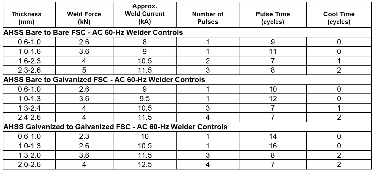
Table 3: AHSS bare-to-bare, bare-to-galvanized, Galvanized-to-galvanized RSW parameters for pulsating AC 60 Hz.A-14
Heat, Material and Thickness Balances
The heat input in Resistance Spot Welding (RSW) is defined as:
Heat Input = I2Rt
where: I is welding current
R is total resistance, and
t is weld time
The heat input must be changed depending on the gauge and grade of the steel. Compared to low strength steel at a particular gauge, the AHSS at the same gauge will need less current. Similarly, the thin gauge material needs less current than thick gauge. Controlling the heat input according to the gauge and grade is called heat balance in RSW.
For constant thickness, Table 1 shows steel classification based on strength level. With increasing group numbers, higher electrode force, longer weld time, and lower current are required for satisfactory RSW. Material combinations with one group difference can be welded with little or no changes in weld parameters. Difference of two or three groups may require special considerations in terms of electrode cap size, force, or type of power source.
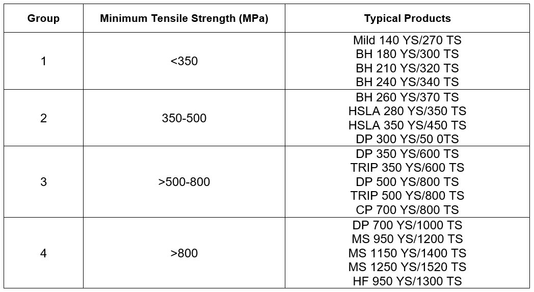
Table 1: Steel classification for RSW purposes.A-11
For a particular steel grade, changes in thickness may require adoption of special schedules to control heat balance. When material type and gauge are varied together, specific weld schedules may need to be developed. Due to the higher resistivity of AHSS, the nugget growth occurs preferentially in AHSS. Electrode life on the AHSS-side may be reduced due to higher temperature on this side. In general, electrode life when welding AHSS may be similar to mild steel because of lower operating current requirement due to higher bulk resistivity in AHSS. This increase in electrode life may be offset in production due to poor part fit up created by higher AHSS springback. Frequent tip dressing will maintain the electrode tip shape and help achieve consistently acceptable quality welds.
Welding Current Mode
AHSS can be welded with power sources operated with either AC or DC types (Figure 1). Middle-Frequency Direct-Current (MFDC) has an advantage over conventional AC due to both unidirectional and continuous current. These characteristics assist in controlling and directing the heat generation at the interface. Current mode has no significant difference in weld quality. It should be noted that both AC and DC can easily produce acceptable welds where thickness ratios are less than 2:1. However, some advantage may be gained using DC where thickness ratios are over 2:1, but welding practices must be developed to optimize the advantages. It also has been observed that nugget sizes are statistically somewhat larger when using DC welding with the same secondary weld parameters than with AC. Some studies have shown that welding with MFDC provides improvements in heat balance and weld process robustness when there is a thickness differential in AHSS (as shown in Figure 2). DC power sources have been reported to provide better power factors and lower power consumption than AC power sources. Specifically, it has been reported that AC requires about 10% higher energy than DC to make the same size weld.L-7
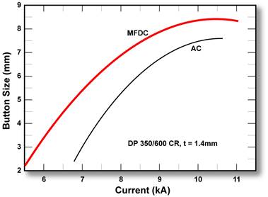
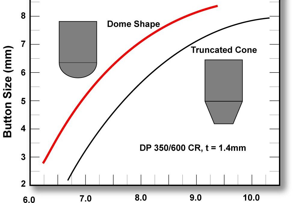
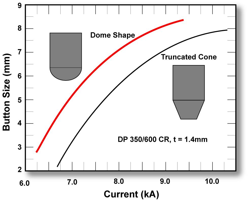
Figure 1: Range for 1.4-mm DP 350/600 CR steel at different current modes with a single pulse.L-2
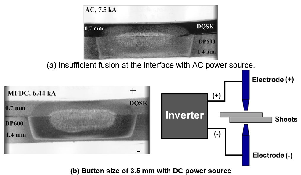
Figure 2: Effect of current mode on dissimilar-thickness stack-up.L-2
Consult safety requirements for your area when considering MFDC welding for manual weld gun applications. The primary feed to the transformers contains frequencies and voltages higher than for AC welding.
Back To Top