Blog, homepage-featured-top, main-blog
Tensile testing is one of the most basic formability characterization methods available. Results from tensile testing are a key input into metal forming simulations, but if the right information isn’t included, the simulation will not accurately reflect material behavior.
Metal forming simulation is particularly beneficial on the value-added parts made from advanced high strength steels, since accurate simulations allow for optimal processing with minimal recuts … at least when the right information is used as inputs.
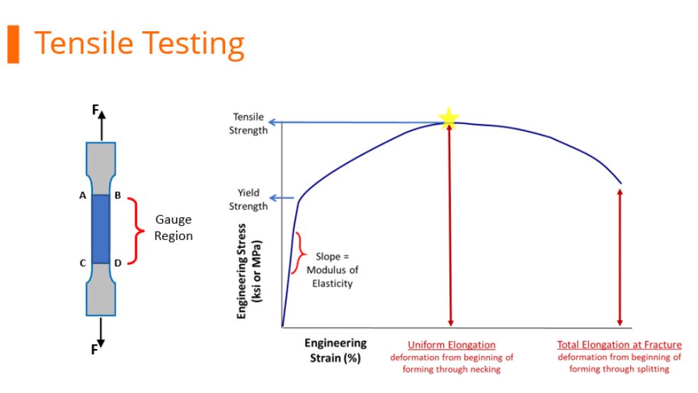
Tensile Testing
During tensile testing, a standard sample shape called a dogbone is pulled in tension. Load and displacement are recorded, and which are then converted to a stress-strain curve. Strength is defined as load divided by cross-sectional area. Exactly when the cross-sectional area is measured during the test influences the results.
Before starting the pull, it’s easiest to measure the width and thickness of the test sample.
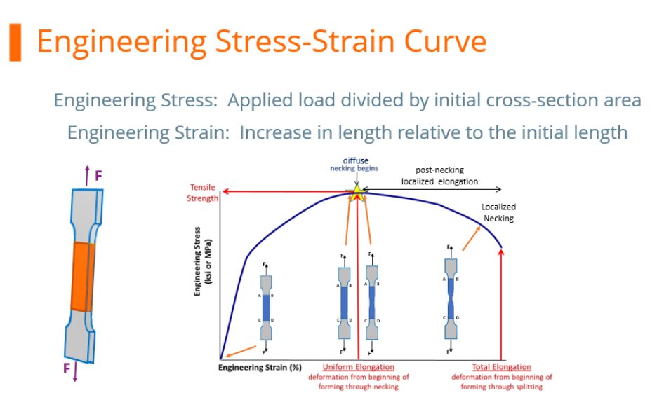
Engineering Stress-Strain Curve
At any load, the engineering stress is the load divided by this initial cross-sectional area. Engineering stress reaches a maximum at the Tensile Strength, which occurs at an engineering strain equal to Uniform Elongation. After that point, engineering stress decreases with increasing strain, progressing until the sample fractures.
However, metals get stronger with deformation through a process known as strain hardening or work hardening. As a tensile test progresses, additional load must be applied to achieve further deformation, even after the “ultimate” tensile strength is reached. Understanding true stress and true strain helps to address the need for additional load after the peak strength is reached.
During the tensile test, the width and thickness shrink as the length of the test sample increases. Although these dimensional changes are not considered when determining the engineering stress, they are of primary importance when determining true stress. At any load, the true stress is the load divided by the cross-sectional area at that instant.
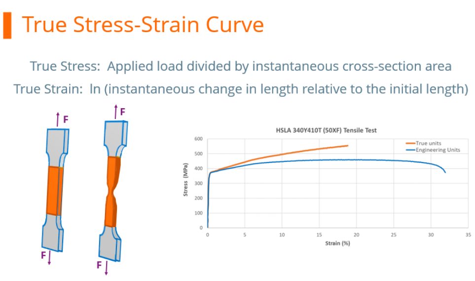
True Stress-Strain Curve
The true stress – true strain curve gives an accurate view of the stress-strain relationship, one where the stress is not dropping after exceeding the tensile strength stress level.
True stress is determined by dividing the tensile load by the instantaneous area.
True stress-strain curves obtained from tensile bars are valid only through uniform elongation due to the effects of necking and the associated strain state on the calculations. Inaccuracies are introduced if the true stress-true strain curve is extrapolated beyond uniform strain, and as such a different test is needed. Biaxial bulge testing has been used to determine stress-strain curves beyond uniform elongation. Optical measuring systems based on the principles of Digital Image Correlation (DIC) are used to measure strains. The method by which this test is performed is covered in ISO 16808.
Stress-strain curves and associated parameters historically were based on engineering units, since starting dimensions are easily measured and incorporated into the calculations. These are the values you see on certified metal properties, also called metal cert sheets that you get with your steel shipments.
True stress and true strain provide a much better representation of how the material behaves as it is being deformed, which explains its use in computer forming and crash simulations.
It’s much more challenging to get accurate dimensional measurements once the test has started unless there are multiple loops of the operator stopping the test, remeasuring, then restarting the pull. This is not a practical approach.
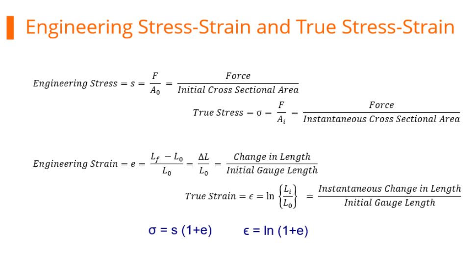
Fortunately, there are equations that relate engineering units to true units. Conventional stress-strain curves generated in engineering units can be converted to true units for inclusion in simulation software packages.
As the industry moves to more value-added stampings, metal forming simulation is done on nearly every part. The value-added nature of parts made from advanced high strength steels requires best practices be used throughout – otherwise the results from simulation drift further away from matching reality, leading to longer development times and costly recuts.

Danny Schaeffler is the Metallurgy and Forming Technical Editor of the AHSS Applications Guidelines available from WorldAutoSteel. He is founder and President of Engineering Quality Solutions (EQS). Danny wrote the monthly “Science of Forming” and “Metal Matters” column for Metalforming Magazine, and provides seminars on sheet metal formability for Auto/Steel Partnership and the Precision Metalforming Association. He has written for Stamping Journal and The Fabricator, and has lectured at FabTech. Danny is passionate about training new and experienced employees at manufacturing companies about how sheet metal properties impact their forming success.

Formability
Strength is defined as load divided by cross-sectional area. In a tensile test, the choice of when the cross-sectional area is measured influences the results.
It is easiest to measure the width and thickness of the test sample before starting the pull. At any load, the engineering stress is the load divided by this initial cross-sectional area. Engineering stress reaches a maximum at the Tensile Strength, which occurs at an engineering strain equal to Uniform Elongation. After that point, engineering stress decreases with increasing strain, progressing until the sample fractures.
However, metals get stronger with deformation through a process known as strain hardening or work hardening. As a tensile test progresses, additional load must be applied to achieve further deformation, even after the “ultimate” tensile strength is reached. Understanding true stress and true strain helps to address the need for additional load after the peak strength is reached.
During the tensile test, the width and thickness shrink as the length of the test sample increases. Although these dimensional changes are not considered in determining the engineering stress, they are of primary importance when determining true stress. At any load, the true stress is the load divided by the cross-sectional area at that instant.
The true stress – true strain curve gives an accurate view of the stress-strain relationship, one where the stress is not dropping after exceeding the tensile strength stress level.
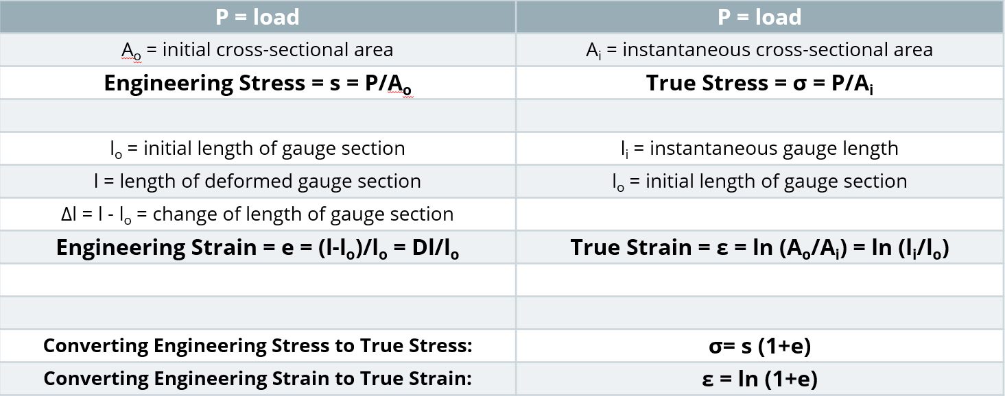
- True stress is determined by dividing the tensile load by the instantaneous area.
- True strain is the natural logarithm of the ratio of the instantaneous gauge length to the original gauge length.
True stress – true strain curves of low carbon steel can be approximated by the Holloman relationship:
σ = Kεn
where true stress = σ; true strain = ε, n is the n-value (work hardening exponent or strain hardening exponent), and the K-value is the true stress at a true strain value of 1.0 (called the Strength Coefficient).
True stress-strain curves obtained from tensile bars are valid only through uniform elongation due to the effects of necking and the associated strain state on the calculations. Inaccuracies are introduced if the true stress-true strain curve is extrapolated beyond uniform strain, and as such a different test is needed. Biaxial bulge testing has been used to determine stress-strain curves beyond uniform elongation. Optical measuring systems based on the principles of Digital Image Correlation (DIC) are used to measure strains. The method by which this test is performed is covered in ISO 16808.I-12
Stress-strain curves and associated parameters historically were based on engineering units, since starting dimensions are easily measured and incorporated into the calculations. True stress and true strain provide a much better representation of how the material behaves as it is being deformed, which explains its use in computer forming and crash simulations. Although sample dimensions are challenging to measure during a tensile test, there are equations that relate engineering units to true units. Conventional stress-strain curves generated in engineering units can be converted to true units for inclusion in simulation software packages.
Relationships Between Engineering and True Properties
More information about the differences between Engineering and True stress-strain curves can be found in the video below, and this blog entry.
![N-Value]()
Mechanical Properties
N-Value, The Strain Hardening Exponent
Metals get stronger with deformation through a process known as strain hardening or work hardening, resulting in the characteristic parabolic shape of a stress-strain curve between the yield strength at the start of plastic deformation and the tensile strength.
Work hardening has both advantages and disadvantages. The additional work hardening in areas of greater deformation reduces the formation of localized strain gradients, shown in Figure 1.

Figure 1: Higher n-value reduces strain gradients, allowing for more complex stampings. Lower n-value concentrates strains, leading to early failure.
Consider a die design where deformation increased in one zone relative to the remainder of the stamping. Without work hardening, this deformation zone would become thinner as the metal stretches to create more surface area. This thinning increases the local surface stress to cause more thinning until the metal reaches its forming limit. With work hardening the reverse occurs. The metal becomes stronger in the higher deformation zone and reduces the tendency for localized thinning. The surface deformation becomes more uniformly distributed.
Although the yield strength, tensile strength, yield/tensile ratio and percent elongation are helpful when assessing sheet metal formability, for most steels it is the n-value along with steel thickness that determines the position of the forming limit curve (FLC) on the forming limit diagram (FLD). The n-value, therefore, is the mechanical property that one should always analyze when global formability concerns exist. That is also why the n-value is one of the key material related inputs used in virtual forming simulations.
Work hardening of sheet steels is commonly determined through the Holloman power law equation:
 Equation 1
where
σ is the true flow stress (the strength at the current level of strain),
K is a constant known as the Strength Coefficient, defined as the true strength at a true strain of 1,
ε is the applied strain in true strain units, and
n is the work hardening exponent
Rearranging this equation with some knowledge of advanced algebra shows that n-value is mathematically defined as the slope of the logarithmic true stress – true strain curve. This calculated slope – and therefore the n-value – is affected by the strain range over which it is calculated. Typically, the selected range starts at 10% elongation at the lower end to the lesser of uniform elongation or 20% elongation as the upper end. This approach works well when n-value does not change with deformation, which is the case with mild steels and conventional high strength steels.
Conversely, many Advanced High-Strength Steel (AHSS) grades have n-values that change as a function of applied strain. For example, Figure 2 compares the instantaneous n-value of DP 350/600 and TRIP 350/600 against a conventional HSLA350/450 grade. The DP steel has a higher n-value at lower strain levels, then drops to a range similar to the conventional HSLA grade after about 7% to 8% strain. The actual strain gradient on parts produced from these two steels will be different due to this initial higher work hardening rate of the dual phase steel: higher n-value minimizes strain localization.

Figure 2: Instantaneous n-values versus strain for DP 350/600, TRIP 350/600 and HSLA 350/450 steels.K-1
As a result of this unique characteristic of certain AHSS grades with respect to n-value, many steel specifications for these grades have two n-value requirements: the conventional minimum n-value determined from 10% strain to the end of uniform elongation, and a second requirement of greater n-value determined using a 4% to 6% strain range.
Plots of n-value against strain define instantaneous n-values, and are helpful in characterizing the stretchability of these newer steels. Work hardening also plays an important role in determining the amount of total stretchability as measured by various deformation limits like Forming Limit Curves.
Higher n-value at lower strains is a characteristic of Dual Phase (DP) steels and TRIP steels. DP steels exhibit the greatest initial work hardening rate at strains below 8%. Whereas DP steels perform well under global formability conditions, TRIP steels offer additional advantages derived from a unique, multiphase microstructure that also adds retained austenite and bainite to the DP microstructure. During deformation, the retained austenite is transformed into martensite which increases strength through the TRIP effect. This transformation continues with additional deformation as long as there is sufficient retained austenite, allowing TRIP steel to maintain very high n-value of 0.23 to 0.25 throughout the entire deformation process (Figure 2). This characteristic allows for the forming of more complex geometries, potentially at reduced thickness achieving mass reduction. After the part is formed, additional retained austenite remaining in the microstructure can subsequently transform into martensite in the event of a crash, making TRIP steels a good candidate for parts in crush zones on a vehicle.
Necking failure is related to global formability limitations, where the n-value plays an important role in the amount of allowable deformation at failure. Mild steels and conventional higher strength steels, such as HSLA grades, have an n-value which stays relatively constant with deformation. The n-value is strongly related to the yield strength of the conventional steels (Figure 3).

Figure 3: Experimental relationship between n-value and engineering yield stress for a wide range of mild and conventional HSS types and grades.K-2
N-value influences two specific modes of stretch forming:
- Increasing n-value suppresses the highly localized deformation found in strain gradients (Figure 1).
A stress concentration created by character lines, embossments, or other small features can trigger a strain gradient. Usually formed in the plane strain mode, the major (peak) strain can climb rapidly as the thickness of the steel within the gradient becomes thinner. This peak strain can increase more rapidly than the general deformation in the stamping, causing failure early in the press stroke. Prior to failure, the gradient has increased sensitivity to variations in process inputs. The change in peak strains causes variations in elastic stresses, which can cause dimensional variations in the stamping. The corresponding thinning at the gradient site can reduce corrosion life, fatigue life, crash management and stiffness. As the gradient begins to form, low n-value metal within the gradient undergoes less work hardening, accelerating the peak strain growth within the gradient – leading to early failure. In contrast, higher n-values create greater work hardening, thereby keeping the peak strain low and well below the forming limits. This allows the stamping to reach completion.
- The n-value determines the allowable biaxial stretch within the stamping as defined by the forming limit curve (FLC).
The traditional n-value measurements over the strain range of 10% – 20% would show no difference between the DP 350/600 and HSLA 350/450 steels in Figure 2. The approximately constant n-value plateau extending beyond the 10% strain range provides the terminal or high strain n-value of approximately 0.17. This terminal n-value is a significant input in determining the maximum allowable strain in stretching as defined by the forming limit curve. Experimental FLC curves (Figure 4) for the two steels show this overlap.

Figure 4: Experimentally determined Forming Limit Curves for mils steel, HSLA 350/450, and DP 350/600, each with a thickness of 1.2mm.K-1
Whereas the terminal n-value for DP 350/600 and HSLA 350/450 are both around 0.17, the terminal n-value for TRIP 350/600 is approximately 0.23 – which is comparable to values for deep drawing steels (DDS). This is not to say that TRIP steels and DDS grades necessarily have similar Forming Limit Curves. The terminal n-value of TRIP grades depends strongly on the different chemistries and processing routes used by different steelmakers. In addition, the terminal n-value is a function of the strain history of the stamping that influences the transformation of retained austenite to martensite. Since different locations in a stamping follow different strain paths with varying amounts of deformation, the terminal n-value for TRIP steel could vary with both part design and location within the part. The modified microstructures of the AHSS allow different property relationships to tailor each steel type and grade to specific application needs.
Methods to calculate n-value are described in Citations A-43, I-14, J-13.
![N-Value]()
Mechanical Properties
Total Elongation to Fracture
Deformation continues in the local neck until fracture occurs. The amount of additional strain that can be accommodated in the necked region depends on the microstructure. Inclusions, particles, and grain boundary cracking can accelerate early fracture. Total elongation is measured from start of deformation to start of fracture. Two extensometer gauge lengths are commonly used: A50 (50mm or 2 inches) and A80 (80 mm).
In the past, limited automation and measurement equipment necessitated the use of a non-repeatable technique defined in ASTM E8A-24 and ISO 6892-1I-7 as “elongation after fracture.” Here, the operator attempts to position the two fractured strips back together and hand measures the distance between two gauge marks on the sample.
Tensile testing combined with data acquisition systems are much more commonplace today. According to ASTM E8, the elongation at fracture shall be taken as the strain measured just prior to when the force falls below 10 % of the maximum force encountered during the test. Both elastic strains and plastic strains are included in the measurement.

Figure 1 : Total elongation is measured from start of deformation to start of fracture.
![N-Value]()
Mechanical Properties
Engineering stress-strain units are based on the starting dimensions of the tensile test sample: Engineering stress is the load divided by the starting cross-sectional area, and engineering strain is the change in length relative to the starting gauge length (2 inches, 50mm, or 80mm for ASTM [ISO I], JIS [ISO III], or DIN [ISO II] tensile test samples, respectively.)
Metals get stronger with deformation through a process known as strain hardening or work hardening. This is represented on the stress strain curve by the parabolic shaped section after yielding.
Concurrent with the strengthening as the tensile test sample elongates is the reduction in the width and thickness of the test sample. This reduction is necessary to maintain consistency of volume of the test sample.
Initially the positive influence of the strengthening from work hardening is greater than the negative influence of the reduced cross-section, so the stress-strain curve has a positive slope. As the influence of the cross-section reduction begins to overpower the strengthening increase, the stress-strain curve slope approaches zero.
When the slope is zero, the maximum is reached on the vertical axis of strength. This point is known as the ultimate tensile strength, or simply the tensile strength. The strain at which this occurs is known as uniform elongation.
Strain concentration after uniform elongation results in the formation of diffuse necks and local necks and ultimately fracture.
Figure 1: Tensile Strength is the Strength at the Apex of the Engineering Stress – Engineering Strain Curve.