1stGen AHSS, AHSS, Steel Grades
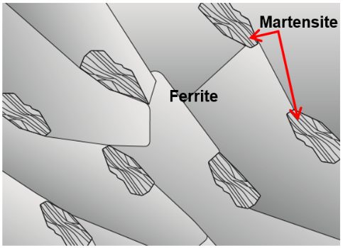
Dual Phase (DP) steels have a microstructure consisting of a ferritic matrix with martensitic islands as a hard second phase, shown schematically in Figure 1. The soft ferrite phase is generally continuous, giving these steels excellent ductility. When these steels deform, strain is concentrated in the lower-strength ferrite phase surrounding the islands of martensite, creating the unique high initial work-hardening rate (n-value) exhibited by these steels. Figure 2 is a micrograph showing the ferrite and martensite constituents.
Figure 1: Schematic of a Dual Phase steel microstructure showing islands of martensite in a matrix of ferrite.
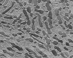
Figure 2: Micrograph of Dual Phase Steel
Hot rolled DP steels do not have the benefit of an annealing cycle, so the dual phase microstructure must be achieved by controlled cooling from the austenite phase after exiting the hot strip mill finishing stands and before coiling. This typically requires a more highly alloyed chemistry than cold rolled DP steels require. Higher alloying is generally associated with a change in welding practices.
In one possible approach, after exiting the last finishing stand of the hot rolling mill, controlled cooling facilitates the nucleation of ferrite. Then a more rapid cooling fast enough to avoid bainite formation is needed to reach the Ms (martensite start) temperature and begin nucleating martensite from the austenite that had not transformed to ferrite.
Continuously annealed cold-rolled and hot-dip coated Dual Phase steels are produced by controlled cooling from the two-phase ferrite plus austenite (α + γ) region to transform some austenite to ferrite before a rapid cooling transforms the remaining austenite to martensite. Due to the production process, small amounts of other phases (bainite and retained austenite) may be present.
Higher strength dual phase steels are typically achieved by increasing the martensite volume fraction. Depending on the composition and process route, steels requiring enhanced capability to resist cracking on a stretched edge (as typically measured by hole expansion capacity) can have a microstructure containing significant quantities of bainite.
The work hardening rate plus excellent elongation creates DP steels with much higher ultimate tensile strengths than conventional steels of similar yield strength. Figure 3 compares the engineering stress-strain curve for HSLA steel to a DP steel curve of similar yield strength. The DP steel exhibits higher initial work hardening rate, higher ultimate tensile strength, and lower YS/TS ratio than the HSLA with comparable yield strength. Additional engineering and true stress-strain curves for DP steel grades are presented in Figures 4 and 5.
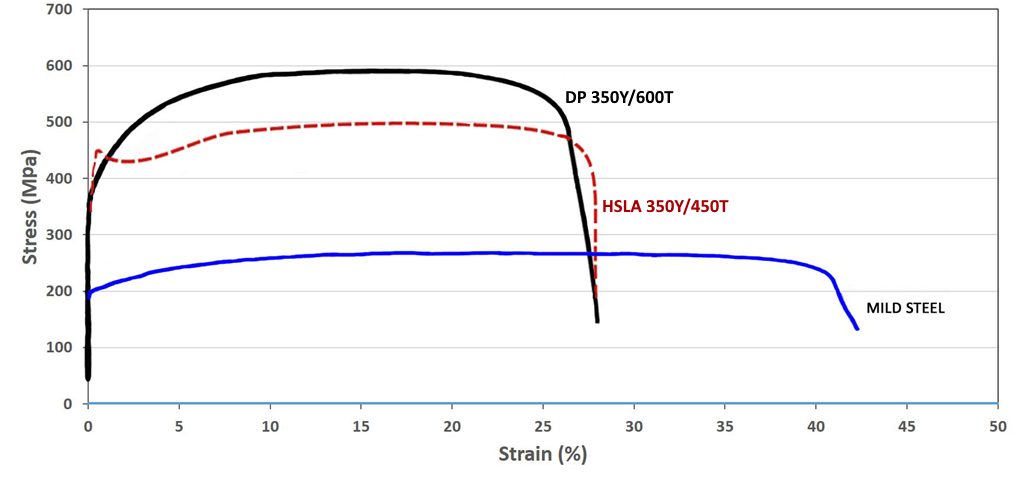
Figure 3: A comparison of stress strain curves for mild steel, HSLA 350/450, and DP 350/600K-1

Figure 4: Engineering stress-strain curves for a series of DP steel grades.S-5, V-1 Sheet thicknesses: DP 250/450 and DP 500/800 = 1.0mm. All other steels were 1.8-2.0mm.

Figure 5: True stress-strain curves for a series of DP steel grades.S-5, V-1 Sheet thicknesses: DP 250/450 and DP 500/800 = 1.0mm. All other steels were 1.8-2.0mm.
The volume fraction, morphology, and distribution of the martensite in the ferrite matrix is responsible for the mechanical properties of dual phase (DP) steels. The intercritical annealing temperature, cooling rate, and alloy content affect the martensite volume fraction in the finished product.
Martensite can have different appearances (morphologies) in the microstructure including needle-like, granular, and equiaxed, and these impact the strength and ductility of DP steels. The most favorable balance of strength and ductility usually is associated with a uniform distribution of equiaxed martensite islands.
These properties influence the hole expansion ratio, which measures the expandability of a sheared edge. The amount of carbon in martensite controls martensite hardness relative to the ferrite, and a greater hardness difference between martensite and ferrite is associated with decreased HER values.
The number of martensite colonies per unit area has a positive correlation with sheared edge stretchability, indicating that there is a greater dispersion of these islands of this high-hardness phase. A more homogeneous microstructure is known to have better HER and sheared-edge formability properties.T-57.
Although dual phase steels are more formable than HSLA steels at the same tensile strength, there is a greater risk of cut edge fractures forming and propagating during stretch flanging. This is due to the hardness difference between the ferrite and martensite phases.
In these steels, micro-voids form at the interface between the soft phase and hard phase at the sheared edge (Figure 6), and can fracture during flanging under tension. Reducing the hardness difference of the microstructural components is one approach to improve edge fracture resistance, which is one of the merits of using complex phase steels.

Figure 6: Microstructure at the punched edge of a DP steel.M-75
DP and other AHSS also have a bake hardening effect that is an important benefit compared to conventional higher strength steels. The extent of the bake hardening effect in AHSS depends on an adequate amount of forming strain for the specific chemistry and thermal history of the steel.
In DP steels, carbon enables the formation of martensite at practical cooling rates by increasing the hardenability of the steel. Manganese, chromium, molybdenum, vanadium, and nickel, added individually or in combination, also help increase hardenability. Carbon also strengthens the martensite as a ferrite solute strengthener, as do silicon and phosphorus. These additions are carefully balanced, not only to produce unique mechanical properties, but also to maintain the generally good resistance spot welding capability. However, when welding the higher strength grades (DP 700/1000 and above) to themselves, the spot weldability may require adjustments to the welding practice.
Dual Phase Steel for Exposed Panels
In recent decades, bake hardenable steels have been a common choice for outer surface panels. Many of these applications center around grades with yield strength of approximately 200 MPa and tensile strength below approximately 400 MPa. Work hardening (strengthening occurring from forming) combined with bake hardening (strengthening from the paint curing cycle during automotive production) usually adds around 70 to 100 MPa to the yield strength, enhancing the dent resistance of these panels.
To further support the lightweighting efforts of the automobile industry, steelmakers have developed dual phase steels with appropriate surface characteristics for exposed panel applications. The benefits of deploying dual phase steels in these applications include a higher yield strength from the steel mill (300 MPa minimum yield strength) and a greater strengthening increase from bake hardening (typically more than 100 MPa) in addition to the work hardening from forming. The strengthening increase allows the automaker to downgauge the sheet thickness to as low as 0.55 mm and maintain adequate dent resistance. More information on the bake hardenability of exposed quality dual phase steels can be found here.
The primary grade in this category can be described as HC300/500DPD+Z, where HC indicates that it is high strength cold rolled steel, 300/500 represents the minimum yield and tensile strength in MPa, DPD is “dual phase deep drawing,” and Z indicates that it is galvanized.
The stress-strain curves of HC300/500DPD+Z are compared with those of common traditional bake hardening grades used for automotive outer skin panels in Figures 7 and 8. The comparison of engineering stress-strain curves are shown in Figure 7, with Figure 8 comparing the true stress-strain curves.
The dual phase steel exhibits a higher tensile strength and greater work hardening (n-value) – especially in the 4% to 6% range that coincides with the strain range associated with stamping automotive outer panels.
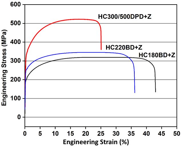
Figure 7: Engineering stress-strain curves for 0.6 mm HC300Y/500T-DPD+Z (galvanized 500 DP in red), 0.75 mm HC220BD+Z (galvanized 220 BH in blue), and 0.65 mm HC180BD+Z (galvanized 180 BH in black).
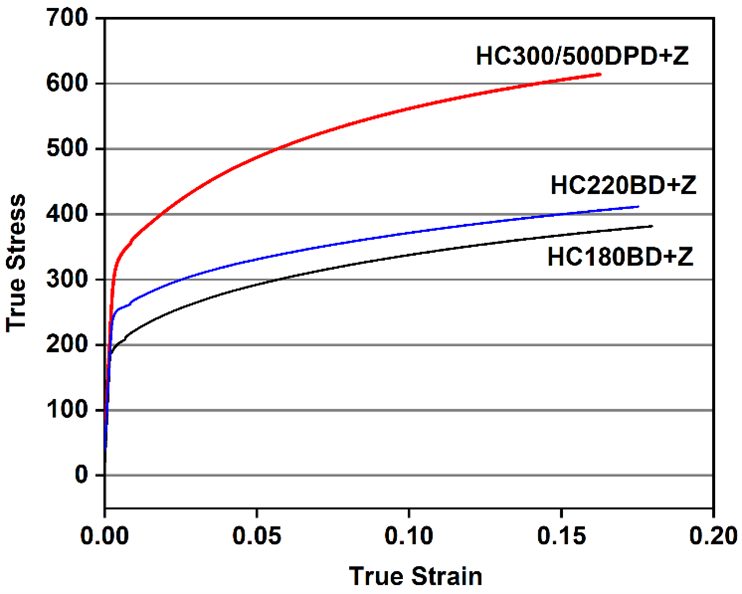
Figure 8: True stress-strain curves for 0.6 mm HC300Y/500T-DPD+Z (galvanized 500 DP in red), 0.75 mm HC220BD+Z (galvanized 220 BH in blue), and 0.65 mm HC180BD+Z (galvanized 180 BH in black).
Figure 9 compares the forming limit curve for HC300/500DPD+Z steel to those of the typical bake hardenable grades. The dual phase grade has comparable to slightly less necking resistance than HC220BD+Z, a bake hardenable steel with 220 MPa minimum tensile strength. The necking resistance of HC180BD+Z is greater than both other grades.
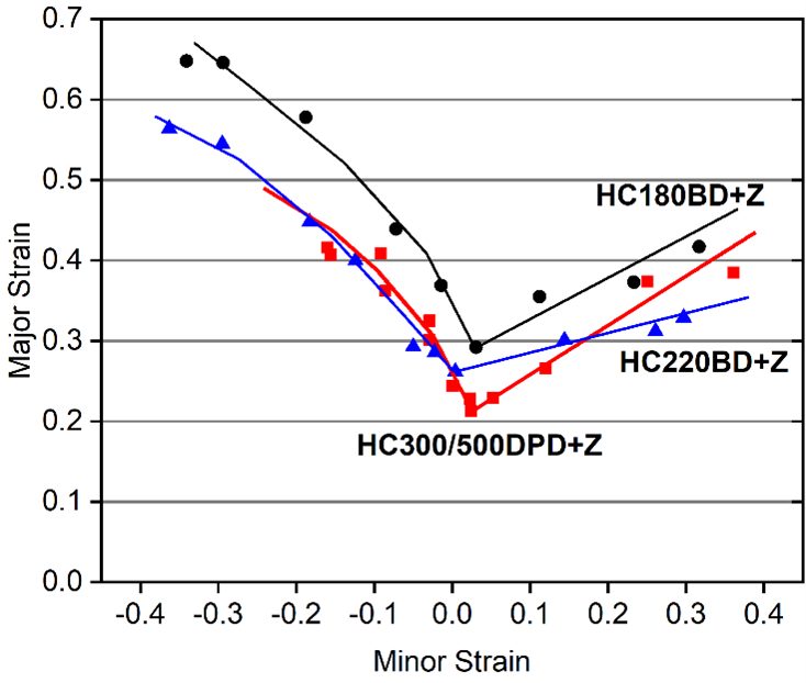
Figure 9: Forming limit curves for 0.6 mm HC300Y/500T-DPD+Z (galvanized 500 DP in red), 0.75 mm HC220BD+Z (galvanized 220 BH in blue), and 0.65 mm HC180BD+Z (galvanized 180 BH in black).
While the thickness reduction offered by HC300/500DPD+Z benefits lightweighting, there is also an associated loss of stiffness. This reduced stiffness typically limits how thin automakers will specify for surface panels, rather than steel mill capabilities.
However, the lower stiffness, higher yield strength, and lower formability negatively influence dimensional accuracy and may contribute to welding challenges. Many of these challenges can be addressed virtually using metal forming simulation.
Examples of current production grades of DP steels and typical automotive applications include:
| DP 300/500 |
Roof outer, door outer, body side outer, package tray, floor panel |
| DP 350/600 |
Floor panel, hood outer, body side outer, cowl, fender, floor reinforcements |
| DP 500/800 |
Body side inner, quarter panel inner, rear rails, rear shock reinforcements |
| DP 600/980 |
Safety cage components (B-pillar, floor panel tunnel, engine cradle, front sub-frame package tray, shotgun, seat) |
| DP 700/1000 |
Roof rails |
| DP 800/1180 |
B-Pillar upper |
Some of the specifications describing uncoated cold rolled 1st Generation dual phase (DP) steel are included below, with the grades typically listed in order of increasing minimum tensile strength and ductility. Different specifications may exist which describe hot or cold rolled, uncoated or coated, or steels of different strengths. Many automakers have proprietary specifications which encompass their requirements.
- ASTM A1088, with the terms Dual phase (DP) steel Grades 440T/250Y, 490T/290Y, 590T/340Y, 780T/420Y, and 980T/550YA-22
- EN 10338, with the terms HCT450X, HCT490X, HCT590X, HCT780X, HCT980X, HCT980XG, and HCT1180XD-6
- JIS G3135, with the terms SPFC490Y, SPFC540Y, SPFC590Y, SPFC780Y and SPFC980YJ-3
- JFS A2001, with the terms JSC590Y, JSC780Y, JSC980Y, JSC980YL, JSC980YH, JSC1180Y, JSC1180YL, and JSC1180YHJ-23
- VDA 239-100, with the terms CR290Y490T-DP, CR330Y590T-DP, CR440Y780T-DP, CR590Y980T-DP, and CR700Y980T-DPV-3
- SAE J2745, with terms Dual Phase (DP) 440T/250Y, 490T/290Y, 590T/340Y, 6907/550Y, 780T/420Y, and 980T/550YS-18
1stGen AHSS, 3rdGen AHSS, AHSS, Steel Grades
topofpage
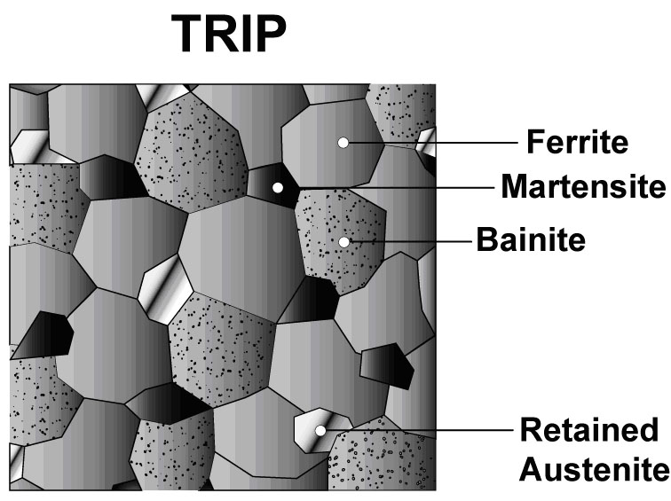
The microstructure of Transformation Induced Plasticity (TRIP) steels contains a matrix of ferrite, with retained austenite, martensite, and bainite present in varying amounts. Production of TRIP steels typically requires the use of an isothermal hold at an intermediate temperature, which produces some bainite. Higher silicon and carbon content of TRIP steels result in significant volume fractions of retained austenite in the final microstructure. Figure 1 shows a schematic of TRIP steel microstructure, with Figure 2 showing a micrograph of an actual sample of TRIP steel. Figure 3 compares the engineering stress-strain curve for HSLA steel to a TRIP steel curve of similar yield strength.
Figure 1: Schematic of a TRIP steel microstructure showing a matrix of ferrite, with martensite, bainite and retained austenite as the additional phases.
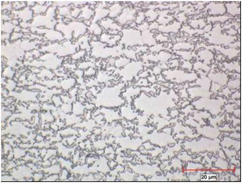
Figure 2: Micrograph of Transformation Induced Plasticity steel.
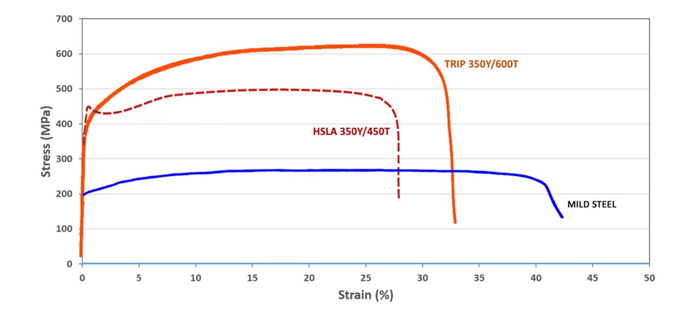
Figure 3: A comparison of stress strain curves for mild steel, HSLA 350/450, and TRIP 350/600.K-1
During deformation, the dispersion of hard second phases in soft ferrite creates a high work hardening rate, as observed in the DP steels. However, in TRIP steels the retained austenite also progressively transforms to martensite with increasing strain, thereby increasing the work hardening rate at higher strain levels. This is known as the TRIP Effect. This is illustrated in Figure 4, which compares the engineering stress-strain behavior of HSLA, DP and TRIP steels of nominally the same yield strength. The TRIP steel has a lower initial work hardening rate than the DP steel, but the hardening rate persists at higher strains where work hardening of the DP begins to diminish. Additional engineering and true stress-strain curves for TRIP steel grades are shown in Figure 5.
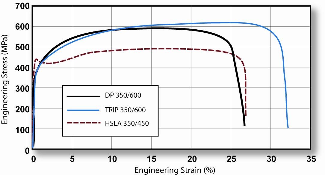
Figure 4: TRIP 350/600 with a greater total elongation than DP 350/600 and HSLA 350/450. K-1
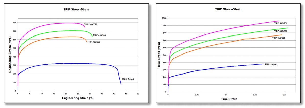
Figure 5: Engineering stress-strain (left graphic) and true stress-strain (right graphic) curves for a series of TRIP steel grades. Sheet thickness: TRIP 350/600 = 1.2mm, TRIP 450/700 = 1.5mm, TRIP 500/750 = 2.0mm, and Mild Steel = approx. 1.9mm. V-1
The strain hardening response of TRIP steels are substantially higher than for conventional HSS, resulting in significantly improved formability in stretch deformation. This response is indicated by a comparison of the n-value for the grades. The improvement in stretch formability is particularly useful when designers take advantage of the improved strain hardening response to design a part utilizing the as-formed mechanical properties. High n-value persists to higher strains in TRIP steels, providing a slight advantage over DP in the most severe stretch forming applications.
Austenite is a higher temperature phase and is not stable at room temperature under equilibrium conditions. Along with a specific thermal cycle, carbon content greater than that used in DP steels are needed in TRIP steels to promote room-temperature stabilization of austenite. Retained austenite is the term given to the austenitic phase that is stable at room temperature.
Higher contents of silicon and/or aluminum accelerate the ferrite/bainite formation. These elements assist in maintaining the necessary carbon content within the retained austenite. Suppressing the carbide precipitation during bainitic transformation appears to be crucial for TRIP steels. Silicon and aluminum are used to avoid carbide precipitation in the bainite region.
The carbon level of the TRIP alloy alters the strain level at which the TRIP Effect occurs. The strain level at which retained austenite begins to transform to martensite is controlled by adjusting the carbon content. At lower carbon levels, retained austenite begins to transform almost immediately upon deformation, increasing the work hardening rate and formability during the stamping process. At higher carbon contents, retained austenite is more stable and begins to transform only at strain levels beyond those produced during forming. At these carbon levels, retained austenite transforms to martensite during subsequent deformation, such as a crash event.
TRIP steels therefore can be engineered to provide excellent formability for manufacturing complex AHSS parts or to exhibit high strain hardening during crash deformation resulting in excellent crash energy absorption.
The additional alloying requirements of TRIP steels degrade their resistance spot-welding behavior. This can be addressed through weld cycle modification, such as the use of pulsating welding or dilution welding. Table 1 provides a list of current production grades of TRIP steels and example automotive applications:
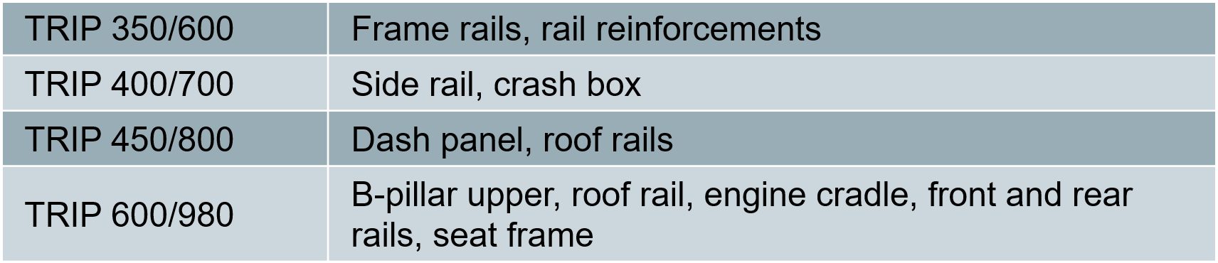
Table 1: Current Production Grades Of TRIP Steels And Example Automotive Applications.
Some of the specifications describing uncoated cold rolled 1st Generation transformation induced plasticity (TRIP) steel are included below, with the grades typically listed in order of increasing minimum tensile strength and ductility. Different specifications may exist which describe hot or cold rolled, uncoated or coated, or steels of different strengths. Many automakers have proprietary specifications which encompass their requirements.
• ASTM A1088, with the terms Transformation induced plasticity (TRIP) steel Grades 690T/410Y and 780T/440YA-22
• JFS A2001, with the terms JSC590T and JSC780TJ-23
• EN 10338, with the terms HCT690T and HCT780TD-18
• VDA 239-100, with the terms CR400Y690T-TR and CR450Y780T-TRV-3
• SAE J2745, with terms Transformation Induced Plasticity (TRIP) 590T/380Y, 690T/400Y, and 780T/420YS-18
Transformation Induced Plasticity Effect
Austenite is not stable at room temperature under equilibrium conditions. An austenitic microstructure is retained at room temperature with the combined use of a specific chemistry and controlled thermal cycle.
Deformation from sheet forming or from crash impact provides the necessary energy to allow the crystallographic structure to change from austenite to martensite. There is insufficient time and temperature for substantial diffusion of carbon to occur from carbon-rich austenite, which results in a high-carbon (high strength) martensite after transformation. Strengthening also occurs from the dislocations formed in the adjacent ferrite required to accommodate the volume increase associated with the austenite-to-martensite transformation.
Transformation to high strength martensite continues as deformation increases, as long as retained austenite (RA) is still available to be transformed. Optimal combinations of strength and ductility are obtained when the retained austenite stability is such that the transformation to martensite occurs gradually with increasing strain.
Alloys capable of the TRIP effect are characterized by a high ductility – high strength combination. Such alloys include 1st Gen AHSS TRIP steels, as well as several 3rd Gen AHSS grades like TRIP-Assisted Bainitic Ferrite, Carbide Free Bainite, and Quench & Partition Steels.
In these grades, increasing the stability of the retained austenite phase delays the austenite-to-martensite transformation to higher strain levels, further promoting formability improvements.
Several factors may promote higher RA stability, including additions of carbon (C) and manganese (Mn). Smaller austenite grains lower the martensite start temperature (Ms) and the number of martensite nucleation sites in each grain, and as such more energy (strain) is needed to start the transformation.
Additions of silicon (Si), chromium (Cr), and aluminum (Al) are also beneficial to achieving the TRIP effect since each of these elements suppress cementite (iron carbide, Fe3C) formation and thereby allows for carbon enrichment of austenite.
However, Mn, Si, Cr, and Al all form oxides on the steel surface that hinder galvanizing and paintability associated with the e-coat layer. Steelmakers typically choose an alloy development and processing strategy which minimizes the detrimental effects of these oxides.
Temperature also has an effect, not only from the paint-bake temperatures of approximately 170 °C, but from galvanizing at close to 500 °C. Citation Z-20 studied the effects of temperature on 0.1%C-5%Mn Medium Manganese steels and found that while tensile strength was relatively independent with temperature, ductility slightly decreases as the temperature is raised from room temperature to 400 °C, but drops off substantially by 500 °C. To retain the formability benefits associated with RA grades, the article recommends galvanizing at temperatures below 400 °C.
In addition to the paint-bake and galvanizing temperatures, adiabatic heating from forming (including shearing and stamping) impact properties. The temperature during forming can be influenced by the starting ambient temperature, the plastic energy dissipation, the latent heat of transformation and by conduction and convection to the environment.M-76
While deforming a metal, most of the energy is dissipated in the form of heat while only a small amount is stored. Austenite-to-martensite transformation kinetics are highly influenced by temperature, and the heating effects associated with mechanically-induced transformation can lead to a severe reduction in ductility.
The temperature rise due to dissipation is not negligible and since the TRIP effect is extremely sensitive to temperature, there is a need for a model to predict this behavior well. Such a model is described in Citation M-76, which reviews that retained austenite stability is a function of several parameters such as temperature; carbon content and alloying elements; austenite grain size and morphology; austenite grain orientation and distribution within the microstructure; and hydrostatic pressure.
Back to the Top
![N-Value]()
Mechanical Properties
N-Value, The Strain Hardening Exponent
Metals get stronger with deformation through a process known as strain hardening or work hardening, resulting in the characteristic parabolic shape of a stress-strain curve between the yield strength at the start of plastic deformation and the tensile strength.
Work hardening has both advantages and disadvantages. The additional work hardening in areas of greater deformation reduces the formation of localized strain gradients, shown in Figure 1.

Figure 1: Higher n-value reduces strain gradients, allowing for more complex stampings. Lower n-value concentrates strains, leading to early failure.
Consider a die design where deformation increased in one zone relative to the remainder of the stamping. Without work hardening, this deformation zone would become thinner as the metal stretches to create more surface area. This thinning increases the local surface stress to cause more thinning until the metal reaches its forming limit. With work hardening the reverse occurs. The metal becomes stronger in the higher deformation zone and reduces the tendency for localized thinning. The surface deformation becomes more uniformly distributed.
Although the yield strength, tensile strength, yield/tensile ratio and percent elongation are helpful when assessing sheet metal formability, for most steels it is the n-value along with steel thickness that determines the position of the forming limit curve (FLC) on the forming limit diagram (FLD). The n-value, therefore, is the mechanical property that one should always analyze when global formability concerns exist. That is also why the n-value is one of the key material related inputs used in virtual forming simulations.
Work hardening of sheet steels is commonly determined through the Holloman power law equation:
 Equation 1
where
σ is the true flow stress (the strength at the current level of strain),
K is a constant known as the Strength Coefficient, defined as the true strength at a true strain of 1,
ε is the applied strain in true strain units, and
n is the work hardening exponent
Rearranging this equation with some knowledge of advanced algebra shows that n-value is mathematically defined as the slope of the logarithmic true stress – true strain curve. This calculated slope – and therefore the n-value – is affected by the strain range over which it is calculated. Typically, the selected range starts at 10% elongation at the lower end to the lesser of uniform elongation or 20% elongation as the upper end. This approach works well when n-value does not change with deformation, which is the case with mild steels and conventional high strength steels.
Conversely, many Advanced High-Strength Steel (AHSS) grades have n-values that change as a function of applied strain. For example, Figure 2 compares the instantaneous n-value of DP 350/600 and TRIP 350/600 against a conventional HSLA350/450 grade. The DP steel has a higher n-value at lower strain levels, then drops to a range similar to the conventional HSLA grade after about 7% to 8% strain. The actual strain gradient on parts produced from these two steels will be different due to this initial higher work hardening rate of the dual phase steel: higher n-value minimizes strain localization.

Figure 2: Instantaneous n-values versus strain for DP 350/600, TRIP 350/600 and HSLA 350/450 steels.K-1
As a result of this unique characteristic of certain AHSS grades with respect to n-value, many steel specifications for these grades have two n-value requirements: the conventional minimum n-value determined from 10% strain to the end of uniform elongation, and a second requirement of greater n-value determined using a 4% to 6% strain range.
Plots of n-value against strain define instantaneous n-values, and are helpful in characterizing the stretchability of these newer steels. Work hardening also plays an important role in determining the amount of total stretchability as measured by various deformation limits like Forming Limit Curves.
Higher n-value at lower strains is a characteristic of Dual Phase (DP) steels and TRIP steels. DP steels exhibit the greatest initial work hardening rate at strains below 8%. Whereas DP steels perform well under global formability conditions, TRIP steels offer additional advantages derived from a unique, multiphase microstructure that also adds retained austenite and bainite to the DP microstructure. During deformation, the retained austenite is transformed into martensite which increases strength through the TRIP effect. This transformation continues with additional deformation as long as there is sufficient retained austenite, allowing TRIP steel to maintain very high n-value of 0.23 to 0.25 throughout the entire deformation process (Figure 2). This characteristic allows for the forming of more complex geometries, potentially at reduced thickness achieving mass reduction. After the part is formed, additional retained austenite remaining in the microstructure can subsequently transform into martensite in the event of a crash, making TRIP steels a good candidate for parts in crush zones on a vehicle.
Necking failure is related to global formability limitations, where the n-value plays an important role in the amount of allowable deformation at failure. Mild steels and conventional higher strength steels, such as HSLA grades, have an n-value which stays relatively constant with deformation. The n-value is strongly related to the yield strength of the conventional steels (Figure 3).

Figure 3: Experimental relationship between n-value and engineering yield stress for a wide range of mild and conventional HSS types and grades.K-2
N-value influences two specific modes of stretch forming:
- Increasing n-value suppresses the highly localized deformation found in strain gradients (Figure 1).
A stress concentration created by character lines, embossments, or other small features can trigger a strain gradient. Usually formed in the plane strain mode, the major (peak) strain can climb rapidly as the thickness of the steel within the gradient becomes thinner. This peak strain can increase more rapidly than the general deformation in the stamping, causing failure early in the press stroke. Prior to failure, the gradient has increased sensitivity to variations in process inputs. The change in peak strains causes variations in elastic stresses, which can cause dimensional variations in the stamping. The corresponding thinning at the gradient site can reduce corrosion life, fatigue life, crash management and stiffness. As the gradient begins to form, low n-value metal within the gradient undergoes less work hardening, accelerating the peak strain growth within the gradient – leading to early failure. In contrast, higher n-values create greater work hardening, thereby keeping the peak strain low and well below the forming limits. This allows the stamping to reach completion.
- The n-value determines the allowable biaxial stretch within the stamping as defined by the forming limit curve (FLC).
The traditional n-value measurements over the strain range of 10% – 20% would show no difference between the DP 350/600 and HSLA 350/450 steels in Figure 2. The approximately constant n-value plateau extending beyond the 10% strain range provides the terminal or high strain n-value of approximately 0.17. This terminal n-value is a significant input in determining the maximum allowable strain in stretching as defined by the forming limit curve. Experimental FLC curves (Figure 4) for the two steels show this overlap.

Figure 4: Experimentally determined Forming Limit Curves for mils steel, HSLA 350/450, and DP 350/600, each with a thickness of 1.2mm.K-1
Whereas the terminal n-value for DP 350/600 and HSLA 350/450 are both around 0.17, the terminal n-value for TRIP 350/600 is approximately 0.23 – which is comparable to values for deep drawing steels (DDS). This is not to say that TRIP steels and DDS grades necessarily have similar Forming Limit Curves. The terminal n-value of TRIP grades depends strongly on the different chemistries and processing routes used by different steelmakers. In addition, the terminal n-value is a function of the strain history of the stamping that influences the transformation of retained austenite to martensite. Since different locations in a stamping follow different strain paths with varying amounts of deformation, the terminal n-value for TRIP steel could vary with both part design and location within the part. The modified microstructures of the AHSS allow different property relationships to tailor each steel type and grade to specific application needs.
Methods to calculate n-value are described in Citations A-43, I-14, J-13.
![N-Value]()
Testing and Characterization
topofpage
Tensile testing characterizes the forming and structural behavior of sheet metals. The test involves loading a sample with a well-defined shape along the axis in tension, generally to fracture, and recording the resultant load and displacement to calculate several mechanical properties. Global standardsI-7, A-24, D-19, J-15 prescribe the conditions under which tests must occur.
Sample Size and Shape
Full-size samples for tensile testing of metal sheets have a rectangular section at the edges for gripping by the test machine. Reducing the width in the central area promotes fracture in the monitored region. These geometrical features result in a sample shape which resembles a dogbone, leading to a descriptive term applied to test samples.
Dimensions of the dogbone samples are associated with tensile test standard from which they apply. ISO I, II, and III (described in Citation I-7) corresponds to the ASTMA-24, DIND-19, and JISJ-15 shapes, respectively. Figure 1 shows the dogbone shapes, highlighting the critical dimensions of width and gauge length. Refer to the Test Standards for other dimensions, tolerances, and other requirements.

Figure 1: Full-size tensile sample shapes for ISO I (ASTM), ISO II (DIN), and ISO III (JIS) standards.I-7, A-24, D-19, J-15
Significant differences exist in the width and gauge length of these tensile bar shapes. Although the ASTM and JIS bars have similar gauge length, the width of the JIS bar is twice that the ASTM bar. The ASTM and DIN bars have a 4:1 ratio of gauge length to width, where the JIS bar has a 2:1 ratio.
These shape differences mean that the calculated elongation changes depending on the test-sample standard used, even when testing identical material. With the combination of the shortest gauge length and widest sample, elongation from JIS bars typically are higher than what would be generated from the other shapes.
Yield strength and tensile strength are not a function of the shape of the tensile bar. Strength is defined as the load divided by the cross-sectional area. Even though each of the bars specify a different sample width (and therefore different cross-section), the load is normalized by this value, which negates differences from sample shape.
Shearing or punching during sample preparation may work-harden the edges of the tensile bar, which may lead to generating an inaccurate representation of the mechanical properties of the sheet metal. Test Standards require subsequent machining or other methods to remove edge damage created during sample preparation. Milling or grinding the dogbone samples minimizes the effects sample preparation may have on the results.
Tensile Test Procedure
The gauge length is the reference length used in the elongation calculations. Depending on the test standard, the gauge length is either 2 inches, 80 mm, or 50 mm. Multiplying the width and thickness within the gauge length determines the initial cross-sectional area before testing.
Grips tightly clamp the edges of the sample at opposite ends. As the test progresses, the grips move away from each other at a prescribed rate or in response to the restraining load. A load cell within the grips or load frame monitors force. An extensometer tracks displacement within the gauge length. Samples are typically tested until fracture.
During the tensile test, the sample width and thickness shrink as the length of the test sample increases. However, these dimensional changes are not considered in determining the engineering stress, which is determined by dividing the load at any time during the test by the starting cross-sectional area. Engineering strain is the increase in length within the gauge length relative to the starting gauge length. (Incorporating the dimensional changes occurring during testing requires calculating true stress and strain. The differences between engineering and true stress/strain are covered elsewhere (hyperlink to 2.3.2.1-Engineering/True)
A graph showing stress on the vertical axis and strain on the horizontal axis is the familiar engineering stress-strain curve, Figure 2. From the stress-strain curve, numerous parameters important for sheet metal forming appear, including:

Figure 2: Engineering stress-strain curve from which mechanical properties are derived.
Influence of Test Speed
Conventional tensile testing is done at strain rates slow enough to be called “quasi-static.” These rates are several orders of magnitude slower than the deformation rates during stamping, which itself is several orders of magnitude slower than what is experienced during a crash event.
Stress-strain curves change with test speed, typically getting stronger as the speed increases. The magnitude of these changes varies with grade. Significant challenges exist when attempting to characterize the tensile response at higher strain rates. Improved equipment and data collection capabilities are among the required upgrades.
Influence of Tensile Test Equipment
Advanced High-Strength Steels (AHSS) may challenge older test equipment. The load and displacement response must reflect only the contributions of the sheet metal, and not be influenced by the load frame and other testing equipment. In much the same way that insufficiently stiff press crowns deflect when stamping AHSS parts, tensile test load frames may similarly deflect, resulting in inaccuracies in the load-displacement measurements.
Grip strength also becomes critical when testing AHSS samples. The high strength of the metal sheets requires more grip pressure to prevent sample slippage through the grips. Pneumatic grips and even some mechanical grips may not generate the necessary pressure. Hydraulically actuated grips may be necessary as the strength increases.
Back to the Top