Blog, homepage-featured-top, main-blog
Efficient energy and resource use in automotive engineering is a major challenge that can only be overcome with innovative solutions. A cost-effective and resource-saving approach is the use of digital methods in production.
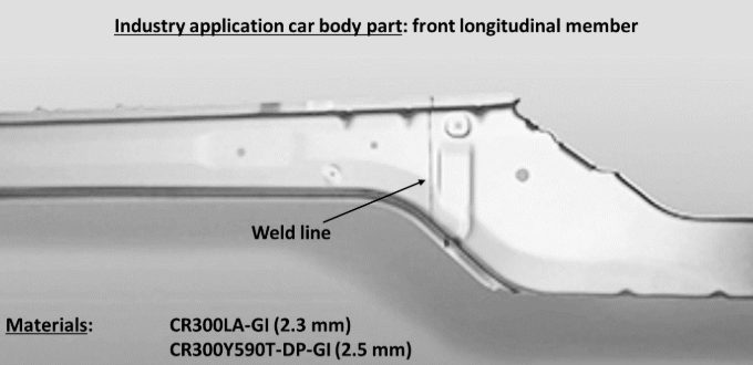
In demanding production chains like body-in-white components from tailor-welded blanks (TWBs), it is crucial to digitally simulate the product before actual production to prevent tool adjustments and unnecessary trials. A new digital twin for the tailor welded blanking process chain links numerical simulations for welding and forming steps. Figure 1 shows a typical application for a tailor welded blank component in the body in white: front longitudinal member.
Figure 1: A typical application for TWBs in the automotive industry is the longitudinal member shown here at the front. The TWB shown consists of micro-alloyed CR300 LA (2.3 mm) and high-strength dual phase steel with 600 MPa (2.5 mm). The welded sheet metal blanks were deep-drawn into the final shape of the TWB.
The process chain of laser beam welding and deep drawing faces challenges when pushing to stronger advanced high-strength steels. Areas around the weld seam are susceptible to softening due to heat input during welding, leading to changes in material properties, such as decreased strength in the heat-affected zone (HAZ) and hardening of the weld metal, influencing forming limit behavior.
Adapted welding process control can optimize material properties, ensuring laser beam welding’s applicability for AHSS grades. Consistent digital simulation of manufacturing processes is one of the most promising approaches for enabling low-emission, lightweight construction and maximizing material efficiency. To replace material-intensive experiments, simulations using the finite element analysis (FEA) create a virtual 3D model of a component.
Welding structure simulation validation is performed using thermocouple measurements and metallographic sections. The core of the forming simulation consists of material cards for high-strength steels. Yield curves, stress-strain curves, and forming limit diagrams are incorporated into the simulation. Validation experiments complete the forming simulation setup, comparing the deep-drawing press force-displacement curve with the modeled curve. The deep-drawn component is then digitized using a 3D scanner, allowing comparison of the real component with the simulated one in terms of geometry, defects, and sheet thickness. Figure 2 shows a simulated S-rail as demonstrator component after deep-drawing simulation.
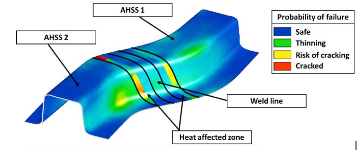
Figure 2: Simulation result of an S-rail formed from TWBs for the probability of failure (max. failure). Both the weld seam and the heat-affected zone are greatly oversized in the illustration for better visibility. The base materials are two high-strength steels of different sheet thicknesses, which were welded together using a butt joint. The heat-affected zone is represented as two areas with different properties.
Today’s forming simulation tools cannot readily account for the small geometric areas of weld metal and heat affected zones, hence the welding simulation results cannot be directly used as input for another software. In addition, it is difficult to measure material behavior of the welding zones to correctly model them in forming simulations. New interfaces were developed for a digital data management platform to bridge this gap. Intermediate steps are required to transfer welding results to forming simulation, including determining the heat-affected zone and deriving weld seam geometry. The analysis chain of the digital twin involves extracting welding simulation results, creating input for forming simulation and adjusting welding simulations based on forming results in an iterative loop. Figure 3 illustrates the digital process chain.
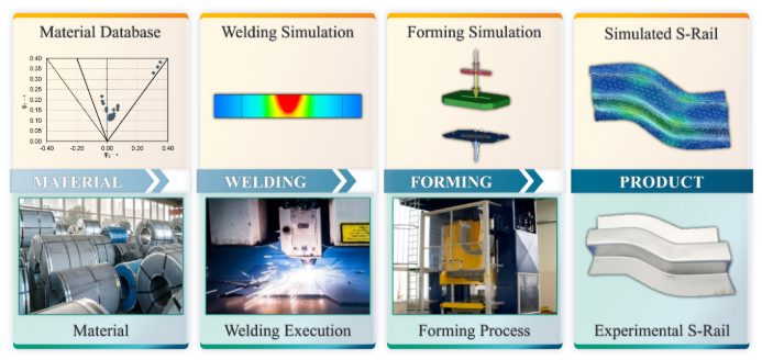
Figure 3: Scheme of the digital (top) and conventional (bottom) process chain of tailor welded blanking: main process steps from material to final product.
Linking welding and forming simulations (Figure 4) enable TWBs made of advanced high-strength steels reach higher strength levels, ultimately saving resources in car body construction and making production more sustainable. The development of TWBs for automotive construction serves as a starting point for expanding lightweight construction potential across the transport sector.
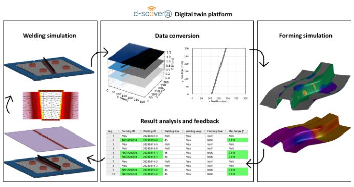
Figure 4: Bidirectional digital twin: How adapting welding simulation closes the loop. The welding simulation displays its results using three-dimensional volume elements. With the help of the digital platform, a simplified two-dimensional representation is generated that contains information about the position of the weld seam and heat-affected zone, which can then be modelled in shell elements. This data is used for the forming simulation and the result is fed back into the digital platform. The parameters of the best simulation results are highlighted and assist in the planning of new welding simulations.

A special thank you to our author, Josefine Lemke, M. Sc. She is a research associate at Fraunhofer IPK in Berlin, Department Joining and Coating Technology. She specialized in additive manufacturing and welding simulation. The focus is on the correlation of component quality and powder properties, particularly in the context of industry and SME environments. She is also working on the qualification of ultra-high-strength steels in car body construction (integration of laser welding and forming simulation in tailor-welded blanking).

Blog, homepage-featured-top, Joining Dissimilar Materials, main-blog
The discussions relative to cold stamping are applicable to any forming operation occurring at room temperature such as roll forming, hydroforming, or conventional stamping. Similarly, hot stamping refers to any set of operations using Press Hardening Steels (or Press Quenched Steels), including those that are roll formed or fluid formed.
Automakers contemplating whether a part is cold stamped or hot formed must consider numerous factors. This blog covers some important considerations related to welding these materials for automotive applications. Most important is the discussion on Resistance Spot Welding (RSW) as it is the dominating process in automotive manufacturing.
Setting Correct Welding Parameters for Resistance Spot Welding
Specific welding parameters need to be developed for each combination of material type and thickness. In general, the Hot Press (HP) steels require more demanding process conditions. One important factor is electrode force which should be higher for the HP steel than for cold press type steel of the same thickness. The actual recommended force will depend on the strength level, and the thickness of the steel. Of course, this will affect the welding machine/welding gun force capability requirement.
Another important variable is the welding current level and even more important is the current range at which acceptable welds can be made. The current range is weldability measurement, and the best indicator of the welding process robustness in the manufacturing environment and sometime called proceed window. Note the relative range of current for different steel types. A smaller process window may require more frequent weld quality evaluation such as for weld size.
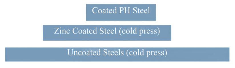
Relative Current Range (process windows) for Different Steel Types
The Effect of Coating Type on Weldability
In all cases of resistance spot welding coated steels, it is imperative to move the coating away from the weld area during and in the beginning of the weld cycle to allow a steel-to-steel weld to occur. The combination of welding current, weld time and electrode force are responsible for this coating displacement.
For all the coated steels, the ability of the coating to flow is a function of the coating type and properties, such as electrical resistivity and melting point, as well as the coating thickness.
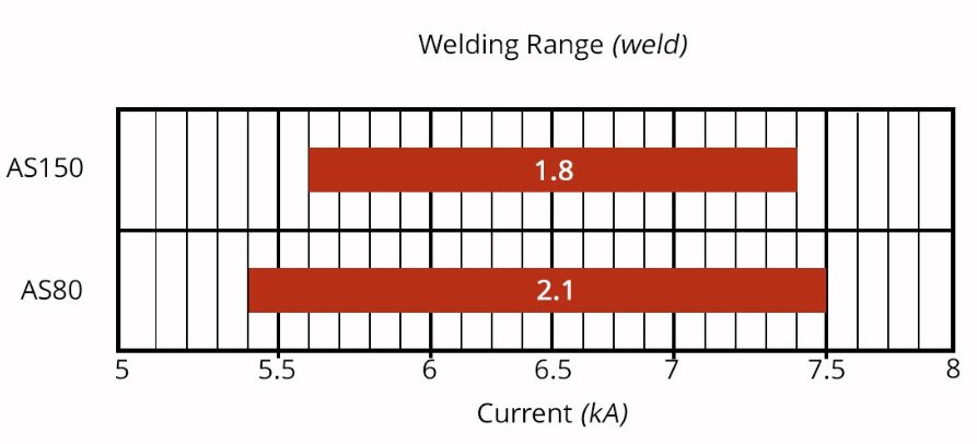
An example of cross sectioned spot welds made on Hot Press Steel with Aluminum -Silicon coating is shown below. It shows two coating thicknesses and the displaced coating at the periphery of weld. This figure also shows the difference in current range for the different coating thickness. The thicker coating shows a smaller current range. In addition, the Al-Si coating has a much higher melting point than the zinc coatings on the cold stamped steels, making it more difficult to displace from the weld area.
Hot Press Steel with Aluminum -Silicon
Liquid Metal Embrittlement and Resistance Spot Welding
Cold-formable, coated, Advance High Strength Steels such as the 3rd Generation Advanced High Strength Steels are being widely used in automotive applications. One welding issue these materials encounter is the increased hardness in the weld area, that sometime results in brittle fracture of the weld.
Another issue is their sensitivity to Liquid Metal Embrittlement (LME) cracking. These two issues are discussed in detail on the WorldAutoSteel AHSS Guidelines website and our recently released Phase 2 Report on LME.
Resistance Spot Welding Using Current Pulsation
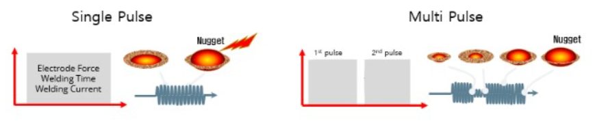
The most effective solution for the issues described above is using current pulsation during the welding cycle. A schematic description is shown below.
The pulsation allows much better control of the heat generation and the weld nugget development. The pulsation variables include the number of pulses (typically 2-4), the current level and time for each pulse, and the cool time between the pulses.
In summery, pulsation (and sometime current upslope) in Resistance Spot Welding proved to be beneficial for the following applications:
- Coated Cold Stamped steels
- Cold stamped Advance High Strength Steels
- Multi materials stack-ups – As described in our articles here on 3T/4T and 5T Stack-Ups

Thanks is given to Menachem Kimchi, Associate Professor-Practice, Dept of Materials Science, Ohio State University and Technical Editor – Joining, AHSS Application Guidelines, for this article.
Blog, homepage-featured-top, Joining, Joining Dissimilar Materials, main-blog, News, Resistance Spot Welding, Resistance Welding Processes, RSW Modelling and Performance, RSW of Dissimilar Steel
This blog is a short summary of a published comprehensive research work titled: “Peculiar Roles of Nickel Diffusion in Intermetallic Compound Formation at the Dissimilar Metal Interface of Magnesium to Steel Spot Welds” Authored by Luke Walker, Carolin Fink, Colleen Hilla, Ying Lu, and Wei Zhang; Department of Materials Science and Engineering, The Ohio State University
*****
There is an increased need to join magnesium alloys to high-strength steels to create multi-material lightweight body structures for fuel-efficient vehicles. Lightweight vehicle structures are essential for not only improving the fuel economy of internal combustion engine automobiles but also increasing the driving range of electric vehicles by offsetting the weight of power systems like batteries.
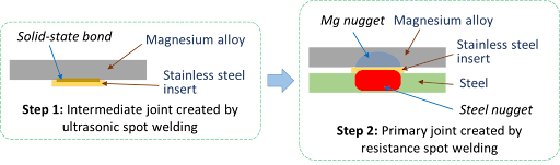
To create these structures, lightweight metals, such as magnesium (Mg) alloys, have been incorporated into vehicle designs where they are joined to high strength steels. It is desirable to produce a metallurgical bond between Mg alloys and steels using welding. However, many dissimilar metal joints form intermetallic compounds (IMCs) that are detrimental to joint ductility and strength. Ultrasonic interlayered resistance spot welding (Ulti-RSW) is a newly developed process that has been used to create strong dissimilar joints between aluminum alloys and high-strength steels. It is a two-step process where the light metal (e.g., Al or Mg alloy) is first welded to an interlayer (or insert) material by ultrasonic spot welding (USW). Ultrasonic vibration removes surface oxides and other contaminates, producing metal-to-metal contact and, consequently, a metallurgical bond between the dissimilar metals. In the second step, the insert side of the light metal is welded to steel by the standard resistance spot welding (RSW) process.
Cross-section View Schematics of Ulti-RSW Process Development
For resistance spot welding of interlayered Mg to steel, the initial schedule attempted was a simple single pulse weld schedule that was based on what was used in our previous study for Ulti-RSW of aluminum alloy to steel . However, this single pulse weld schedule was unable to create a weld between the steel sheet and the insert when joining to Mg. Two alternative schedules were then attempted; both were aimed at increasing the heat generation at the steel-insert interface. The first alternative schedule utilized two current pulses with Pulse 1, high current displacing surface coating and oxides and Pulse 2 growing the nugget. The other pulsation schedule had two equal current pulses in terms of current and welding time.
Lap shear tensile testing was used to evaluate the joint strength using the stack-up schematically, shown below. Note the images of Mg and steel sides of a weld produced by Ulti-RSW.
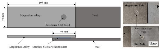 Lap Shear Tensile Test Geometry and the Resultant Weld Nuggets
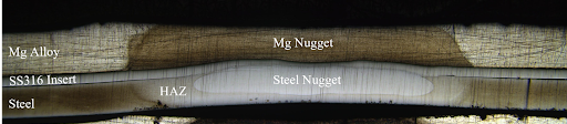
An example of a welded sample showed a distinct feature of the weld that is comprised of two nuggets separated by the insert: the steel nugget formed from the melting of steel and insert and the Mg nugget brazed onto the unmelted insert. This feature is the same as that of the Al-steel weld produced by Ulti-RSW in our previous work. Although the steel nugget has a smaller diameter than the Mg nugget, it is stronger than the latter, so the failure occurred on the Mg sheet side.
Joint strength depends on several factors, including base metal strength, sheet thickness, and nugget size, making it difficult to compare how strong a weld truly is from one process to another. To better compare the dissimilar joints created by different processes, joint efficiency, a “normalized” quantity was calculated for various processes used for dissimilar joining of Mg alloys to steels in the literature, and those results, along with the efficiencies of Ulti-RSW with inserts, are shown together below. Most of the literature studies also used AZ31 as the magnesium base metal. The ones with high joint efficiency (about 53%) in the literature are resistance element welding (REW) and friction stir spot welding (FSSW). In our study, Ulti-RSW with SS316 insert was able to reach an excellent joint efficiency of 71.3%, almost 20% higher than other processes.
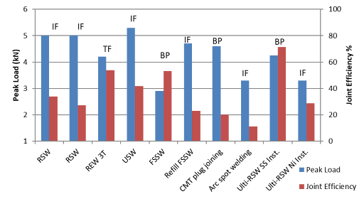 Process Evaluation and Comparison
Thanks are given to Menachem Kimchi, Associate Professor-Practice, Dept of Materials Science, Ohio State University, and Technical Editor – Joining, AHSS Application Guidelines, for this article.
Blog, homepage-featured-top, main-blog, News, Resistance Spot Welding, RSW of Dissimilar Steel, Tool & Die Professionals
Urbanization and waning interest in vehicle ownership point to new transport opportunities in megacities around the world. Mobility as a Service (MaaS) – characterized by autonomous, ride-sharing-friendly EVs – can be the comfortable, economical, sustainable transport solution of choice thanks to the benefits that today’s steel offers.
The WorldAutoSteel organization is working on the Steel E-Motive program, which delivers autonomous ride-sharing vehicle concepts enabled by Advanced High-Strength Steel (AHSS) products and technologies.
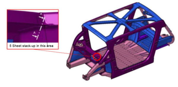
The Body structure design for this vehicle is shown in Figure 1. It also indicates the specific joint configuration of 5 layers AHSS sheet stack-up as shown in Table 1. Resistance spot welding parameters were developed to allow this joint to be made by a single weld. (The previous solution for this welded joint is to create one spot weld with the bottom 3 sheets indicated in the table and a second weld to join the top 2 sheets, combining the two-layer groups to 5T stack-up.)
NOTE: Click this link to read a previous AHSS Insights blog that summarizes development work and recommendations for resistance spot welding 3T and 4T AHSS stack-ups: https://bit.ly/42Alib8
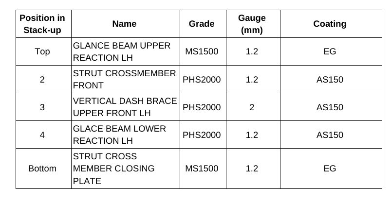
Table 1. Provided materials organized in stack-up formation showing part number, name, grade, gauge in mm, and coating type. Total thickness = 6.8 mm
The same approach of utilizing multiple current pulses with short cool time in between the pulses was shown to be most effective in this case of 5T stack-up. It is important to note that in some cases, the application of a secondary force was shown to be beneficial, however, it was not used in this example.
To establish initial welding parameters simulations were conducted using the Simufact software by Hexagon. As shown in Figure 2, the final setup included a set of welding electrodes that clamped the 5-layer AHSS stack-up. Several simulations were created with a designated set of welding parameters of current, time, number of pulses, and electrode force.
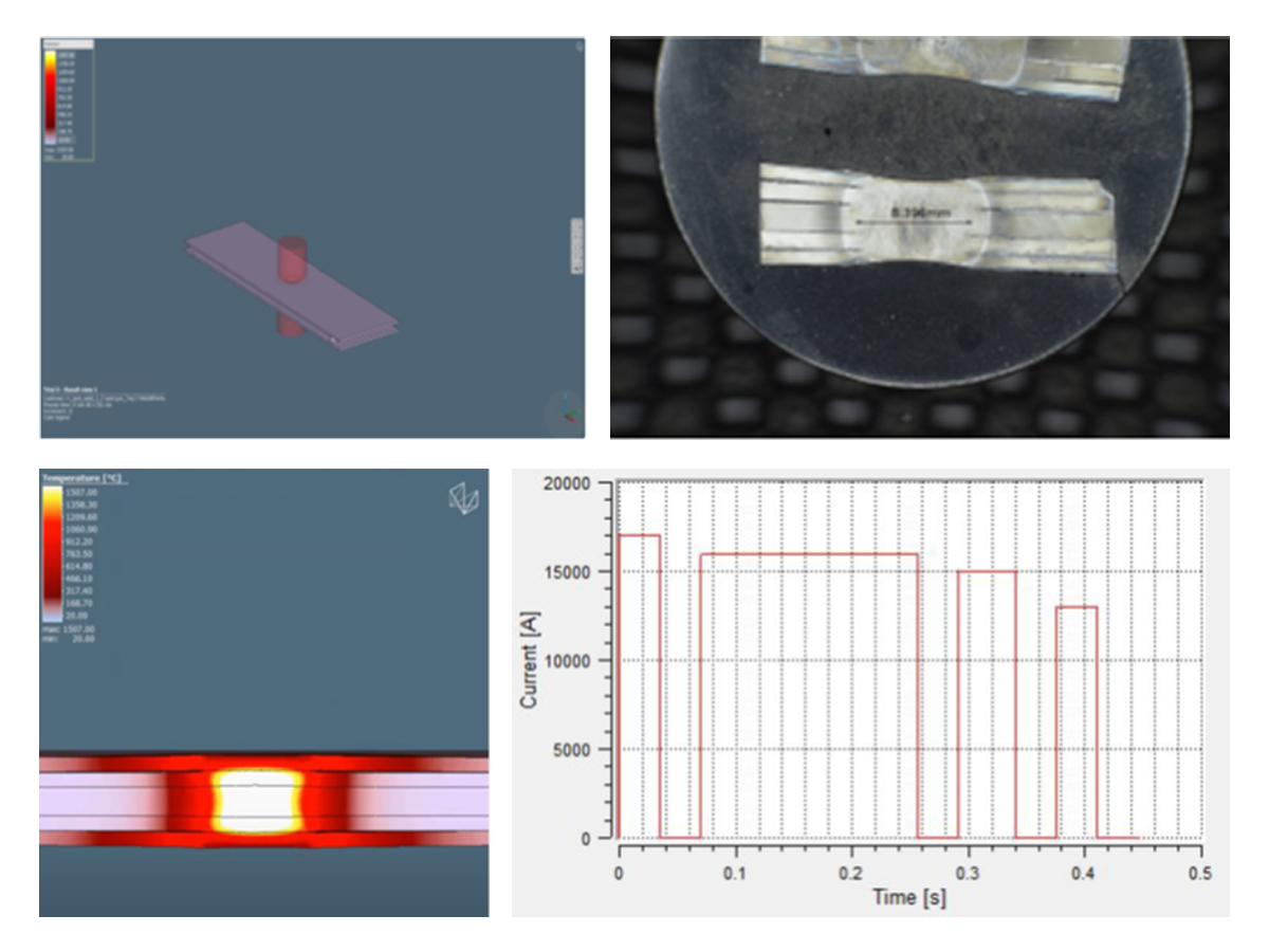
Figure 2. Example of simulation and experimental results showing acceptable 5T resistance spot weld (Meets AWS Automotive specifications)
Thanks is given to Menachem Kimchi, Associate Professor-Practice, Dept of Materials Science, Ohio State University and Technical Editor – Joining, AHSS Application Guidelines, for this article.
Blog, RSW Modelling and Performance
Modern car bodies today are made of increasing volumes of Advanced High-Strength Steels (AHSS), the superb performance of which facilitates lightweighting concepts (see Figure 1). To join the different parts of a car body and create the crash structure, the components are usually welded to achieve a reliable connection. The most prominent welding process in automotive production is resistance spot welding. It is known for its great robustness, and easily applicable in fully automated production lines.
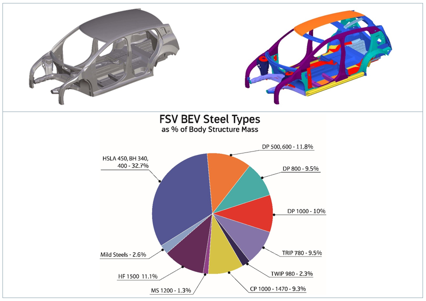
Figure 1: AHSS Content in Modern Car Body.W-7
There are, however, challenges to be met to guarantee a high-quality joint when the boundary conditions change, for example, when new material grades are introduced. Interaction of a liquefied zinc coating and a steel substrate can lead to small surface cracks during resistance spot welding of current AHSS, as shown in Figure 2. This so-called liquid metal embrittlement (LME) cracking is mainly governed by grain boundary penetration with zinc, and tensile stresses. The latter may be induced by various sources during the manufacturing process, especially under ‘rough’ industrial conditions. But currently, there is a lack of knowledge, regarding what is ‘rough’, and what conditions may still be tolerable.
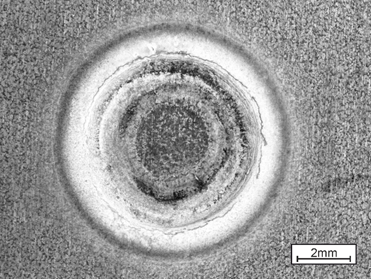
Figure 2: Top View of LME-Afflicted Spot Weld.
The material-specific amount of tensile stresses necessary for LME enforcement can be determined by the experimental procedure ‘welding under external load’. The idea of this method, which is commonly used for comparing cracking susceptibilities of different materials to each other, is to apply increasing levels of tensile stresses to a sample during the welding process and monitor the reaction. Figure 3 shows the corresponding experimental setup.

Figure 3: Welding under external load setup.L-51
However, the known externally applied stresses are not exclusively responsible for LME, but also the welding process itself, which puts both thermally and mechanically induced stresses/strains on the sample. Here, the conventional measuring techniques fail. A numerical reproduction of the experiment grants access to the temperature, stress and strain fields present during the procedure, providing insights on the formation of LME. The electro-thermomechanical simulation model is described in detail in Modelling RSW of AHSS. It is used to simulate the welding under external load procedure (see Figure 4).
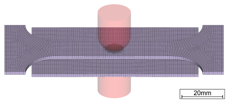
Figure 4: Simulation Model of Welding Under External Load.
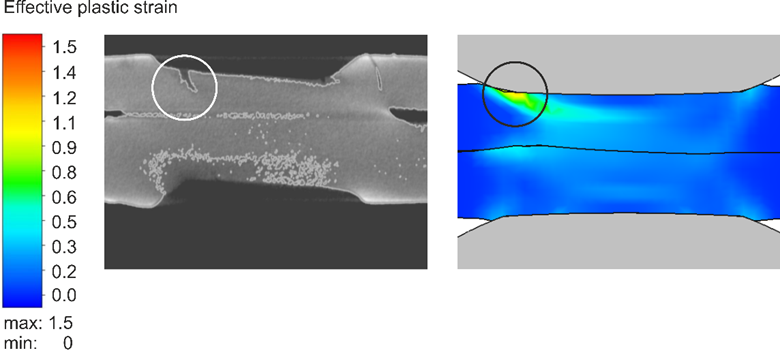
The videos that can be found in the link above show the corresponding temperature and plastic strain fields. As heat dissipates quickly through the water-cooled electrode, a temperature gradient towards the adjacent areas and a local temperature maximum on the surface forms. The plastic strains accumulate mainly at the electrode indentation area. The simulated strain field shows a local maximum of plastic deformation at the left edge of the electrode indentation, amplified by the externally applied stresses and the boundary conditions implied by the procedure. This area correlates with experimentally observed LME cracking sites and paths as shown in Figure 5.
The simulation shows that significant plastic strains are present during welding. When external stresses (in reality e.g. due to poor part fit-up or distorted parts) contribute to the already high load, LME cracking becomes more likely. The numerical simulation model facilitates the determination of material-specific safety limits regarding LME cracking. Parameter variations and their effects on the LME susceptibility can easily be investigated by use of the model, enabling the user to develop strict processing protocols to reduce the likelihood of LME. Finally, these experimental procedures can be adapted to other high-strength materials, to aid their application understanding and industrial set-up conditions.
Figure 5: LME Cracks in Cross Section View at Highly Strained Locations.
For more information on this topic, see the paper, co-authored by Fraunhofer and LWF Paderborn, documented in Citation F-23. You may also download the full report documenting the WorldAutoSteel LME project for which this work was conducted.