B-79
Citations:
B-79. E. Billur and D. Schaeffler, “New Press-Hardening Grades and Process Enhancements for Hot Stamping,” PMA MetalForming Magazine Hot Stamping Experience, 2023.
B-79. E. Billur and D. Schaeffler, “New Press-Hardening Grades and Process Enhancements for Hot Stamping,” PMA MetalForming Magazine Hot Stamping Experience, 2023.
Fundamentals and Principles of Resistance Welding
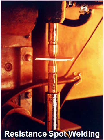
Figure 1: Resistance Spot Welding
Resistance welding processes represent a family of industrial welding processes that produce the heat required for welding through what is known as joule (J = I Rt) heating. Much in the way a piece of wire will heat up when current is passed through it, a resistance weld is based on the heating that occurs due to the resistance of current passing through the parts being welded. Since steel is not a very good conductor of electricity, it is easily heated by the flow of current and is an ideal metal for resistance welding processes. There are many resistance welding processes, but the most common is Resistance Spot Welding (RSW) (Figure 1). All resistance welding processes use three primary process variables – current, time, and pressure (or force). The automotive industry makes extensive use of resistance welding, but it is also used in a variety of other industry sectors including aerospace, medical, light manufacturing, tubing, appliances, and electrical.
In addition to RSW, three other common resistance welding processes are Resistance Seam (RSEW), Projection (RPW), and Flash Welding (RFW) (Figure 2). The RSEW process uses two rolling electrodes to produce a continuous-welded seam between two sheets. It is often the process of choice for welding leak tight seams needed for automotive fuel tanks. RPW relies on geometrical features machined or formed on the part known as projections to create the required weld current density. RFW is very different from the other processes in that it relies on a rapid succession of high-current-density short current pulses which create what is known as flashing. During flashing, molten metal is violently expelled as the parts are moved together. The flashing action heats the surrounding material which allows a weld to be created when the parts are later brought together with significant pressure. Other important resistance welding processes which are not shown include High-Frequency Resistance Welding (HFRW) (used for producing the seams in welded pipe), and Resistance Upset Welding (RUW).
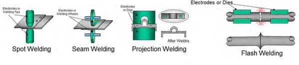
Figure 2: Common resistance welding processes.
In summary, most resistance welding processes offer the following advantages and limitations:
An increasing number of laboratories are using Digital Image Correlation (DIC) to enhance and refine the data captured during testing. DIC is a technique used to measure displacement and deformation using optical and computational tools. Measurement accuracy depends on the proper use of camera, lenses and lighting to capture the movement of a spatter pattern applied to the material sample. Setting up optical equipment requires the operator to understand camera resolution, frame rates, buffering, lens field of view, aperture sizes, depth of field, plane of focus, and the impact of lighting on exposure, shadow, contrast and focus.
The challenges of focusing on a planar surface are different from those of a three-dimensional surface. Where a planar surface can support a ‘focus and shoot’ approach, a 3D surface requires an understanding of depth of field, multi-camera setup and aperture size.
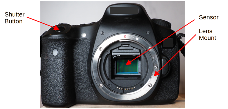
The camera is a dark box that has a mount for a lens and a sensor to capture and store light from the lens image. At its most basic, you can make a camera using film and an oatmeal box with an opaque lid. If you puncture the center of the lid with a pin and mount a piece of film on the back, your oatmeal box camera can capture images. Capturing the image requires you to cover the pinhole with something opaque and remove it until enough light enters the box to expose the film.
Modern cameras operate under the same principles as the oatmeal box. Today’s digital cameras use electronic sensors instead of film and include sophisticated controls to manage:
Figure 1: Key control locations on modern cameras.
There are a number of important considerations when purchasing a camera for use in DIC. Each consideration affects the quality of the images you capture and the accuracy of your displacement measurements.
Higher resolution means greater data capture. This means more detail in the image, but greater data capture means longer times to offload information from the sensor to the buffer, then to data storage. In high-speed photography, lower resolutions can be preferable because data is stored faster and camera buffers can be smaller. Also, large image files take longer to manage and process.
Today’s lenses are precision optical devices. The lens generally manages focus and the volume of light that hits the sensor. Unlike the pinhole camera described above, a lens collects a larger amount of light that can be controlled to manage the quantity of that light which projects on the sensor. The lens can focus on a selected range of subjects. Considerations for selecting a lens include focal length, largest aperture size, and whether it includes a depth of field scale.
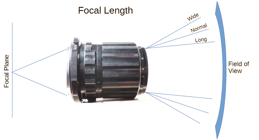
Figure 2: Relationship between focal length and field of view.
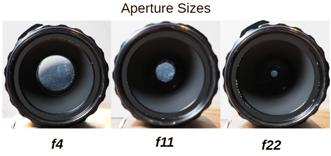
Figure 3: Relative aperture size for 3 f-stops.
The quality of your lighting is arguably the most critical component of your success. There are several types of light sources available. Your goal in lighting is to evenly light the sample surface, provide soft lighting, consistent light output, reduce heat, and color management. Techniques to light your sample properly include:
Two-Dimensional measurement is a single camera setup that works best when the camera is set up perpendicular to the specimen. Although it’s commonly assumed that 2D only supports in-plane surfaces, it can be useful for out-of-plane applications when the deformed specimen remains within the lens’ depth of field.
An advantage of 2D DIC is that it is easy to set up with less hardware. Disadvantages include inaccurate readings when the deformed surface exceeds the lens’ depth of field and it can be affected by perspective distortion introduced by wider lenses.
Three-Dimensional measurement requires two cameras whose fields of view overlap. This setup is ideal for measuring out-of-plane motions, complex geometries and large deformations.
The advantages of 3D measurement include its ability to measure a full 3D shape, displacement and strain fields. Among its disadvantages are the need for continuous camera calibration, the need for a stable stereo camera rig and the need to synchronize image acquisition.
More information about these topics can be found in “A Good Practices Guide for Digital Image Correlation” from International Digital Image Correlation Society, Citation I-26.
 Thanks are given to Bill Frahm, a partner with 4M Partners for his contributions to this page. Bill supports the sheet metal forming industry’s efforts to manage the opportunities and risks of Smart Manufacturing. Sheet metal forming is a fragmented industry. Much of the work forming components is done by small to mid sized manufacturers. These companies are often resource constrained. The latest knowledge about materials, processes, and tools aren’t readily available to employees. Bill’s professional goal is to provide employees with the knowledge and confidence to understand the analysis of smart manufacturing, manage analysis efforts to support their goals, and control data and data products to prevent misuse and bias.
The complex shapes of automotive stampings lead to die designs and processing that may challenge the inherent formability of the selected sheet metal grade.
Traditional grades, especially those of lower strength, fail from insufficient necking resistance for the chosen application. Characterization of the resistance to necking instability, sometimes referred to as global formability, is done with the strain hardening exponent (n-value), true uniform strain, and the Forming Limit Curve. Since these parameters can be mathematically described, forming simulation packages can accurately estimate the risk of necking and subsequent splitting.
Contrast this with newer grades where the sheet metal may still fail from insufficient necking resistance, but may also fail from fracture initiating at cut edges or tight bends. This fracture-limited formability, sometimes called local formability, can be influenced by many parameters – including both inherent material characteristics as well as the processing conditions used to create the cut edge (hole diameter, clearance, punch geometry, and so on) or bend (inside bend radius divided by the thickness, r/t). The inherent material characteristics contributing to this failure mode are not directly related to strength and elongation determined from traditional uniaxial tensile testing. Forming simulation packages have challenges estimating the risk of fracture-limited formability, since the full mathematical representation of the contributing factors does not yet exist.
To date, hole expansion testing is the most common way to characterize the edge stretchability of a particular sheet metal. The typical test procedure, prescribed by ISO 16630, requires a 10 mm diameter hole punched with a 12% clearance to be expanded with a conical punch having a 60° apex angle. Unfortunately, changing the testing conditions like the hole diameter, clearance, punch shape, or crack detection method has a significant influence on the results, to the point that any relative performance ranking of different products can change between the defined laboratory test conditions and the real-world performance.
Local fracture strain measurements from uniaxial tensile specimens, like true fracture strain, true thickness strain, or the reduction of the cross-section area at fracture, are also used to quantify fracture performance, and may offer better guidance for crash performance prediction.L-21, L-69 The bending angle measured from 3-point bending test according to VDA 238-100 or the fracture strain in plane strain tension obtained from these tests, are also effective in predicting bending-dominated failure that occurs with AHSS grades during folding/bending in axial and side crash tests. The bending angle and fracture strain determined in a 3-point bend test conducted according to VDA 238-100 correlates with the folding and bending seen in vehicle crash testing. However, these parameters individually are not sufficient to characterize overall fracture behavior and therefore cannot be used as a singular failure criterion that is applicable to all situations.
Fracture-limited formability is dependent on the sheet metal’s resistance to crack nucleation and propagation, which are the two parameters influencing fracture toughness. As such, approaches have been investigated to experimentally assess the relationship between fracture toughness and cracking resistance of advanced steels.
Conventional toughness estimations based on the product of tensile strength multiplied by the total elongation to fracture (TS * TEL) or the area under the stress-strain curve are not suitable to describe the fracture toughness of AHSS. Use of these shortcuts may lead to an incorrect fracture toughness ranking when considering multiple materials: consider the comparison of 980DP vs. 980CP. The dual phase steel has greater elongation to fracture and greater uniform elongation, yet the complex phase steel has better edge ductility and fracture toughness. Tensile fracture parameters, such as the true fracture strain (εf) or the product of fracture stress and true fracture strain (σf × εf), give a better estimation of toughness at cracking initiation. However, these approaches can underestimate the crack propagation resistance of the material. To avoid misleading conclusions about the cracking resistance of high strength sheet metals, fracture toughness must be measured within the framework of fracture mechanics.F-43
Fracture toughness is defined as the energy spent in the creation of two surfaces at the crack tip that leads to crack propagation. Traditional approaches to study fracture toughness include J-integral and Crack Tip Opening Displacement (CTOD) measurements, but these evaluations do not apply to thin-gauge materials such as those used in automotive body construction. Alternative approaches appropriate for sheets below 3 mm thickness are relatively complex, involve detailed specimen preparation, and require measurement of the advancing crack during the tests.
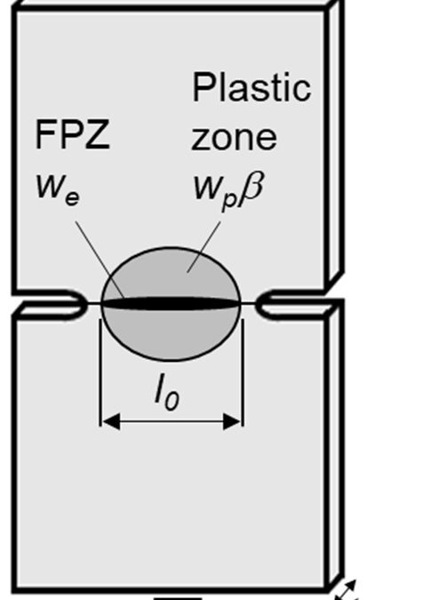
To address these challenges, a methodology based on the Essential Work of Fracture (EWF) appears to offer a simpler solution for measuring the fracture toughness of thin metal sheets. The method described below has been validated in industrial applications using both steel and non-steel sheet metals. The Double Edge Notched Tensile (DENT) specimen is used for this characterization (Figure 1). Since only tensile transverse stresses exist between the notches, and the geometry avoids the risk of buckling.
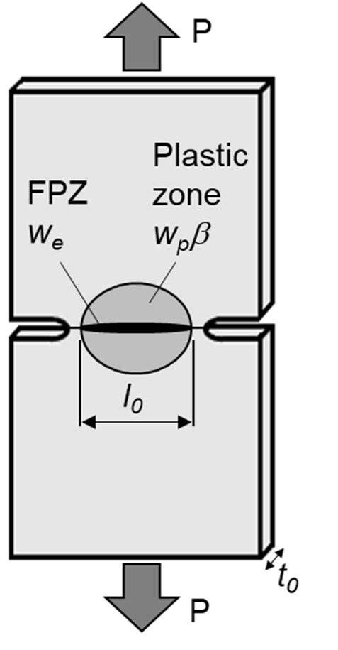
Figure 1: The Double Edge Notched Tensile (DENT) specimen is used for Essential Work of Fracture characterization.
In the DENT specimen, all of the deformation takes place in and around the notched ligament, allowing for separation of the total fracture energy, Wf, into its two components:
a) We, the essential work of fracture that is related to damage and the work to create new surfaces in front of the progressing crack tip. This value is proportional to the fractured area.
b) Wp, the plastic work dissipated in the region surrounding the crack tip as a consequence of plastic deformation. This value is proportional to the deformed volume, which is a function of the sample size, geometry, and loading mode.
Mathematically, the total fracture energy may be represented by:
Wf = We + Wp Equation 1
These parameters can be further characterized.
We = we*l0*t0, where we is the essential work of fracture per unit area, l0 is the ligament length between the two notches, and t0 is the specimen thickness.
Wp = β*wp* l02*t0, where wp is the plastic work per unit volume and β is a shape factor that is a function of the shape of the plastic zone.
Substituting these into Equation 1 gives
Wf = we*l0*t0 + β*wp* l02*t0 Equation 2
Normalizing each side of Equation 2 by the fractured area l0*t0 produces wf, the fracture energy per fracture area:
Wf/ l0*t0 = wf = we + β*wp* l0 Equation 3
This procedure enables the separation of the specific essential work of fracture, we , and the non-essential plastic work, wp, from the total energy of fracture by using a simple data reduction method. A series of specimens with different ligament lengths are tested to fracture. The fracture energy per fracture area, wf, is then calculated by integrating the area under the load-displacement curve and normalizing by the cross-section area (wf= Wf /l0*t0) . . By plotting the series of wf values as a function of ligament length l0 as shown in Figure 2, then we and β*wp can be obtained by linear regression with we being the vertical axis intercept of a line with slope β*wp. It is relevant to keep in mind that this method to obtain we is a purely mathematic procedure to remove the non-essential plastic contribution to the fracture energy, i.e. it does not mean that we is the value of wf at zero ligament length. To guarantee data linearity and the validity of the energy partitioning concept, different validity criteria must be met.T-49
The parameter we is a thickness-dependent material constant representing the plane stress fracture toughness of the material. Since it is obtained from a dataset of energy values for the complete fracture, it contains energetic contributions from both crack initiation and propagation resistance.
For each of the specimens tested with different ligament length, the work of fracture at crack initiation (wfi) is obtained from integrating the area under the load-displacement curve up to the point of crack growth initiation. This point has to be experimentally verified and generally it is around the peak values of the forces versus displacement curve. Since wfi is independent of the ligament length, the specific essential work for fracture initiation, wei can be calculated from an average of wfi values. This is also shown in Figure 2.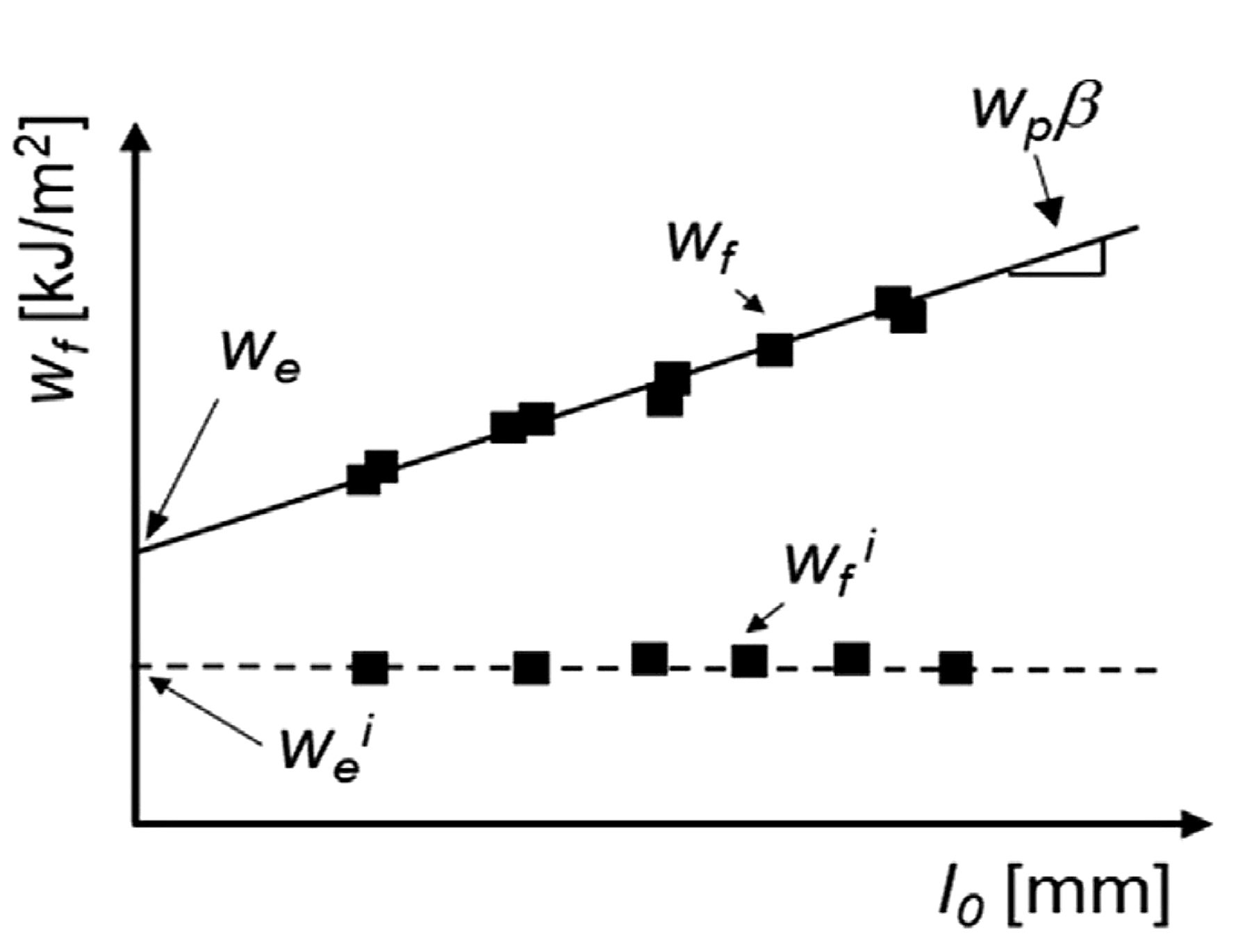
Figure 2: The specific essential work of fracture, we, is the vertical axis intercept in the plot showing the relationship between the specific total work of fracture, wf, and the ligament length. The specific essential work of fracture initiation, wei, is the average of the values of the specific work of fracture at initiation of propagation, wfi.
Figure 3 shows the specific essential work for fracture (we) and specific essential work for fracture initiation (wei) for several advanced high strength steels. The differences between these parameters vary between the grades. For some grades, the markers fall nearly on top of each other, and for these, there is only a small contribution from crack propagation resistance once the crack initiates. For other grades, including complex phase steels and the enhanced-ductility PHS grade, the crack propagation resistance is a significant portion of the overall fracture toughness.
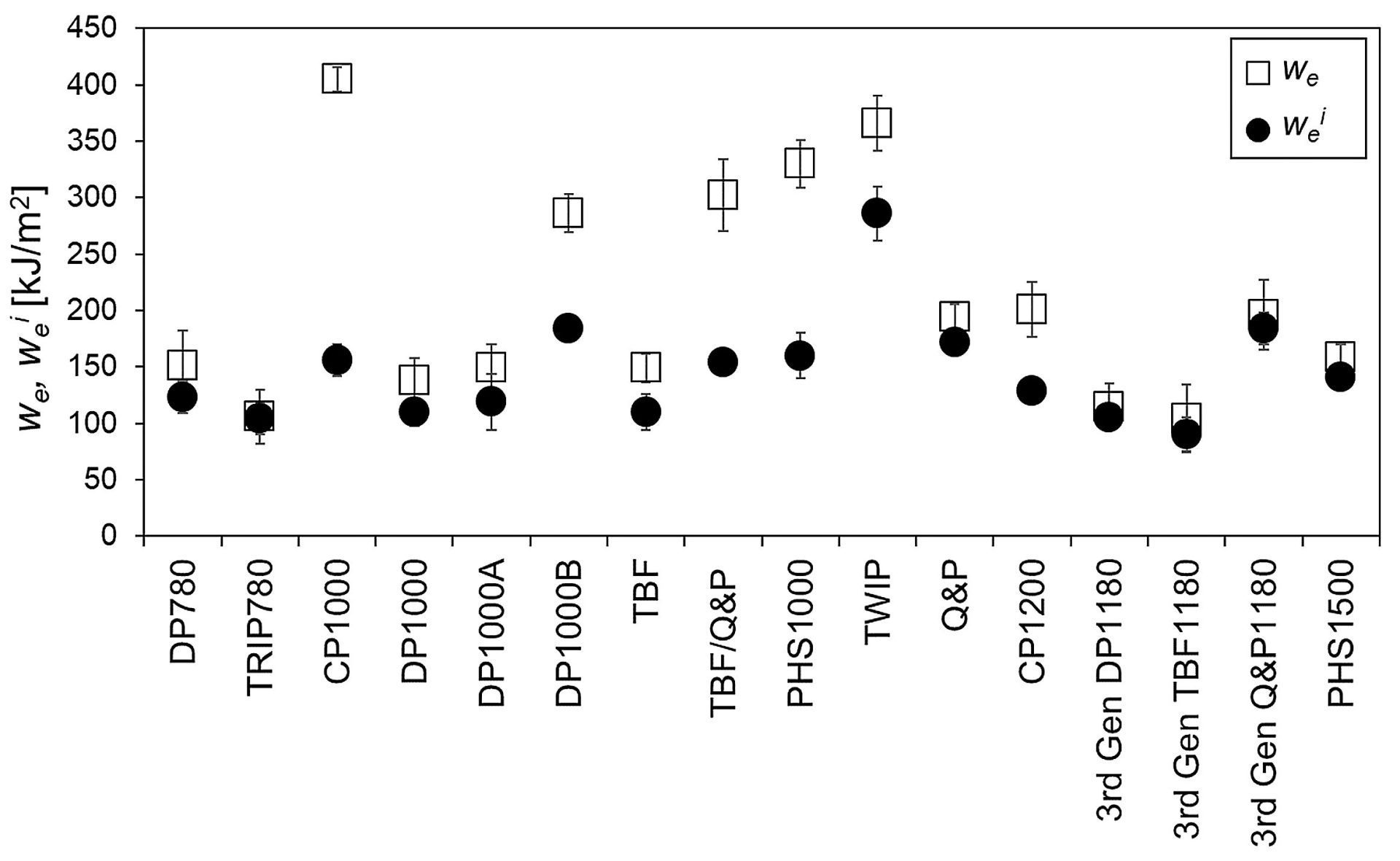
Figure 3: we and wei for several advanced high strength steels. F-44
Notch root radius has a significant influence on EWF measurements. To obtain accurate and reliable fracture toughness values pre-cracked samples must be used. Alternative methods, including fatigue pre-cracking, notch sharpening by a razor blade or mechanical sharp notching with a specific tool, may be used for that purpose. ASTM E399 lists a procedure to nucleate a fatigue crack at the notch rootA-81, as does ASTM E1820A-82. These approaches are relatively costly and time consuming. To address these concerns, a device consisting of a two-pillar modular cutting die and beveled punch was developed to shear sheet specimens in such a manner to introduce crack-like sharp notches.F-45, E-15 Without these efforts to generate an exceedingly small notch radius, the measured toughness values can overestimate the real crack initiation and propagation resistance of the material.F-43
Following the definition of the specific essential work of fracture we , the resistance to crack propagation, it is the material property to address crack-related problems in sheet metal forming, as edge cracking, or to account for part performance when cracks are involved, as in crash resistance tests. In this regard, there is good experimental correlation between the we and the hole expansion ratio for a wide range of AHSS families, as shown in Figure 4. As discussed above, although similarities exist in the fracture mechanisms involved in both tests, the hole expansion ratio is not a material parameter since it depends on several experimental factors such as the hole geometry, edge preparation method, and crack detection method. These choices lead to increased variability of results generated at different labs. Aside from thickness, we is a material property that represents more accurately the sheet steel’s crack propagation resistance. Based on experimental observations a value of we larger than 250 kJ/m2 would be recommended when edge cracking may appear in sheet forming. On the contrary, values lower than 125 kJ/m2 may jeopardize the stamping process.
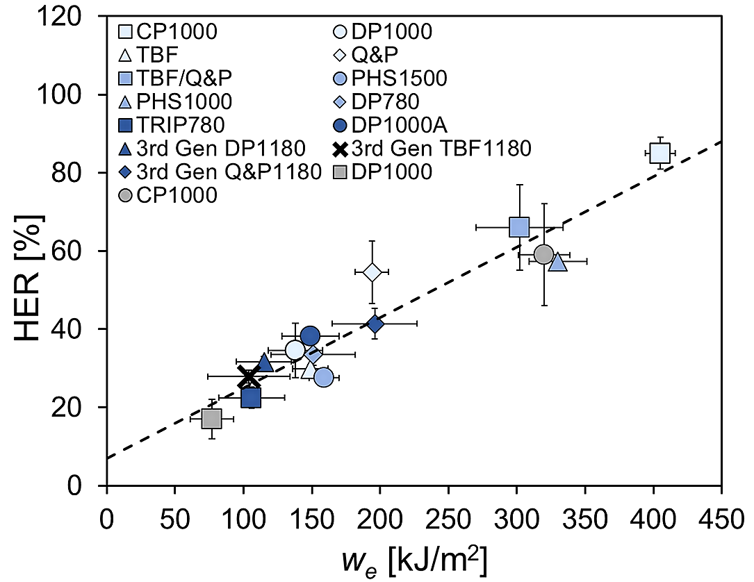
Figure 4: Correlation between we and hole expansion ratio (HER), based on data in Citations F-44, F-46
Crash resistance can be also assessed through the values of the we. In AHSS the appearance of cracks during crash tests ranks crash resistance, so high cracking resistance steel leads to high crashworthiness. The energy absorbed by a component linearly increases with the specific essential work of fracture of the steel used to form the component (Figure 5), making we a good candidate to provide useful information in assessing crashworthiness.F-47
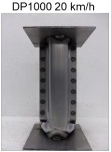 Figure 5a. Crash box made from DP1000 can absorb only limited energy before fracture. F-44 |
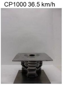 Figure 5b. Crash box made from CP1000 can absorb more energy before fracture.F-44 |
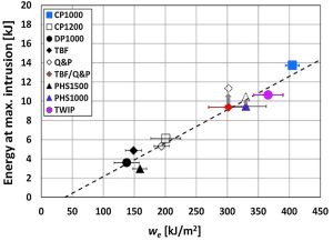 Figure 5c. Energy absorbed at maximum intrusion as a function of the specific essential work of fracture for several advanced steels.F-47 |
Local Formability Diagrams such as the ones shown in Figures 3 and 4 of the Defining Steels page give the user an indication of how a chosen grade might perform in applications requiring fracture resistance, such as those inducing expansion of cut edges during forming. Knowledge of the Essential Work of Fracture offers another representation, as reproduced in Figure 6.F-46 Figure 7 shows a similar representation having tensile strength on the horizontal axis, which is the same format as the conventional Global Formability Diagram.F-48
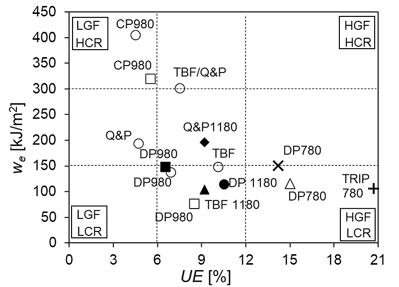
Figure 6: AHSS classification based on uniform elongation (UE, as an indicator of global formability) and fracture resistance (we). LGF low global formability, LCR low cracking resistance, HGF high global formability, HCR high cracking resistance.F-46
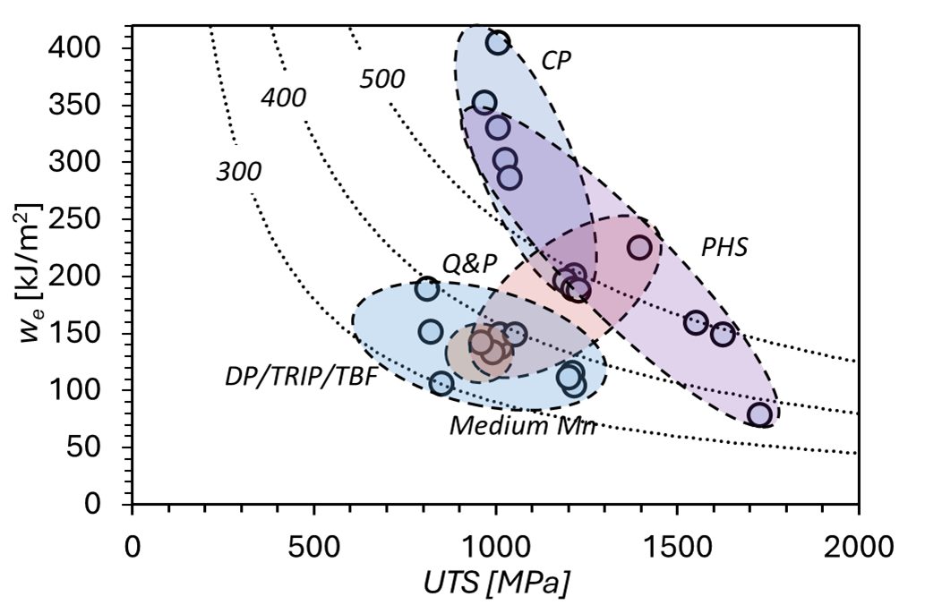
Figure 7: Fracture resistance (we) as a function of tensile strength (UTS) for several Advanced High Strength Steels.F-48
Additional information about the Essential Work of Fracture methodology and its application in fracture toughness, cracking resistance, crashworthiness assessments, User Guidelines, and case studies can be found at https://toughsteel.eu/ as well as Citations C-37, C-38, and C-39.
Thanks are given to David Frómeta and Daniel Casellas of Eurecat for their assistance in preparing this page.

With the rise of electric vehicles, evaluating the environmental impact of each manufacturing process is essential. This article presents an EV battery enclosure welding LCA to compare the sustainability of different joining methods. As automotive manufacturers strive to reduce their carbon footprints, understanding the impact of production processes becomes crucial—especially the joining techniques used in car body assembly. Using Life Cycle Assessment, these impacts can be analyzed in terms of their reduction potential. This article focuses on the example of an all-steel EV battery case joined using several different welding methods.
Life Cycle Assessment is a systematic method for evaluating the environmental impacts of a product or process throughout its life cycle—from raw material extraction to production, use, and disposal. According to DIN EN ISO 14040 standards, LCA is structured into four main components:

Figure 1: Considered system boundaries of the LCA comprising supply of materials and energy, the joining process and disposal of consumables.
The assessed joining processes include:
In the context of joining processes for EV battery cases, this LCA aims to compare the environmental impacts of different welding methods on a meter of weld length. The assessment uses both primary and secondary data from literature and established LCA databases. As not all data is available in-detail for welding processes, several simplifications and assumptions are required:
For example, filler wires aresimplified to pure steel or copper wire rather than taking their complex chemical composition into account. Therefore, it is likely that the actual impact of the filler material production is higher than assumed here. For electricity emissions, the German grid mix is used and to compare resistance spot welding and laser beam welding per weld length, 20 resistance spot welds per meter are assumed.
The emissions from the structural materials are not considered, as the same design is used for all welding processes. Second-order effects due to the switching a joining technology, i.e. the material savings due to reduced flange-widths for laser welding, are also not considered. The second-order material saving effects are known to be larger in comparison to the environmental impact of the joining processes and should be optimized together with the choice of joining process. Further information on these effects can be found in this study.
Figure 2 All-steel EV battery case with zones marked for laser beam and resistance spot welding
The results of the LCA are shown in Figure 3 for the two impact categories Global Warming Potential (i.e. CO2 equivalent emissions) and Acidification Potential (i.e. emission of SO2 equivalent). Main driving factors of emissions are electrical energy, compressed air as well as filler material in the form of steel or copper wire (for laser wire and laser brazing respectively) and adhesive for RSW bonding.
Using the German electrical grid mix, RSW bonding shows the lowest GWP impact. As it does not use any filler material, laser remote welding has the largest potential for CO2 emission reduction, if the electricity generation incorporates more renewable energy .
When analyzing the laser processes, a high idle energy consumption of the laser systems is determined. This is due to the electricity demand of the laser source, cooling and control systems. The consumption only rises slightly, when the lasers are operating. This leads to the conclusion that the overall energy efficiency of laser welding systems can be significantly improved by optimizing “beam-on times” in relation to “idle times”.
In terms of the acidification potential, laser brazing stands out with a far larger impact compared to the other processes, because of the emissions associated with mining and extraction of its copper-based filler material. The wear of copper electrode caps also contributes to this impact category.

Figure 3: Environmental impact of the different welding processes in Global Warming Potential (left) and Acidification (right) per meter of weld length.
Life Cycle Assessment provides invaluable insights into the environmental impacts of joining processes in the automotive industry. By understanding the implications of material choices and energy consumption, manufacturers can make informed decisions that promote sustainability. Both the effect of electricity consumption and filler materials on the environmental impact of automotive joining processes is discussed in this article. Joining processes are one of the major drivers of an OEM’s emissions with ample potential for optimization through LCA analysis.
 |
Thanks go to Dr.-Ing Max Biegler, Group Lead, Joining & Coating Technology Fraunhofer Institute for Production Systems and Design Technology IPK |
Source