RSW Modelling and Performance
This article summarizes the findings of a paper entitled, “Prediction of Spot Weld Failure in Automotive Steels,”L-48 authored by J. H. Lim and J.W. Ha, POSCO, as presented at the 12th European LS-DYNA Conference, Koblenz, 2019.
To better predict car crashworthiness it is important to have an accurate prediction of spot weld failure. A new approach for prediction of resistance spot weld failure was proposed by POSCO researchers. This model considers the interaction of normal and bending components and calculating the stress by dividing the load by the area of plug fracture.
Background
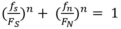
Lee, et al.L-49 developed a model to predict spot welding failure under combined loading conditions using the following equation, based upon experimental results .
|
Equation 1 |
Where FS and FN are shear and normal failure load, respectively, and n is a shape parameter.
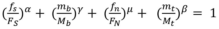
Later, Wung and coworkersW-38 developed a model to predict the failure mode based upon the normal load, shear load, bending and torsion as shown in Equation 2.
 |
Equation 2 |
Here, FS, FN ,Mb and Mt are normal failure load, shear failure load, failure moment and failure torsion of spot weld, respectively. α, β, γ and μ are shape parameters.
Seeger et al.S-106 proposed a model for failure criterion that describes a 3D polynomial failure surface. Spot weld failure occurs if the sum of the components of the normal, bending and shear stresses are above the surface, as shown in the Figure 1.
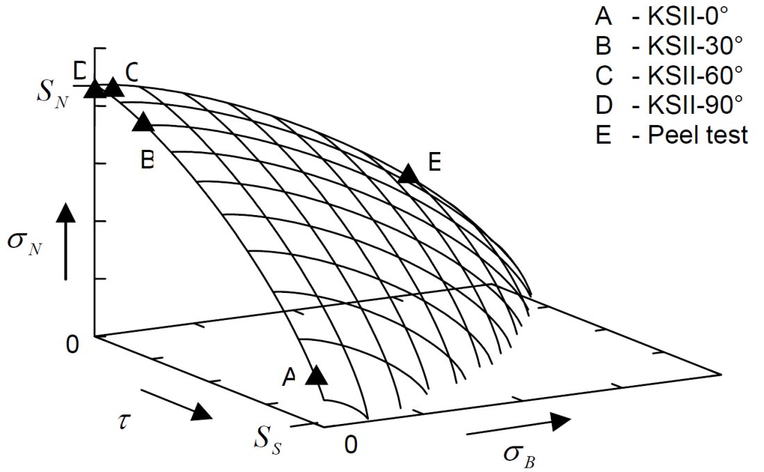
Figure 1: Spot weld failure model proposed by Seeger et al.S-106
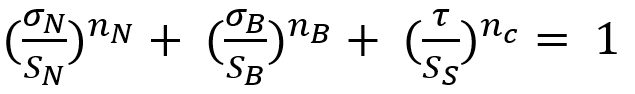
The failure criterion can be expressed via Equation 3.
 |
Equation 3 |
Here, σN , σB , and τ are normal, bending and shear stress of the spot weld, respectively. And nN, nB and nc are the shape parameters. Toyota Motor CorporationL-50 has developed the stress-based failure model as shown in Equation 4.
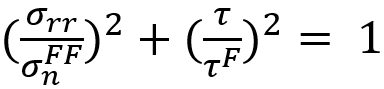 |
Equation 4 |
Hybrid Method to Determine Coefficients for Failure Models
This work used a unique hybrid method to determine the failure coefficients for modeling. The hybrid procedure steps are as follows:
- Failure tests are performed with respect to loading conditions.
- Finite element simulations are performed for each experiment.
- Based on the failure loads obtained in each test, the instant of onset of spot weld failure is determined. Failure loads are extracted comparing experiments with simulations.
- Post processing of those simulations gives the failure load components acting on spot welds such as normal, shear and bending loads.
These failure load components are plotted on the plane consisting of normal, shear and bending axes.
The hybrid method described above is shown in Figure 2.L-48
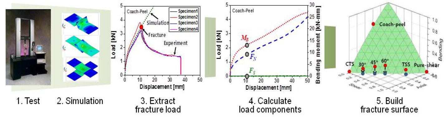
Figure 2: Hybrid method to obtain the failure load with respect to test conditions.L-48
New Spot Weld Failure Model
The new proposed spot weld failure model in this paper considers only plug fracture mode as a normal spot weld failure. Secondly normal and bending components considered to be dependent upon each other. Stress generated by normal and bending components is shear, and shear component generates normal stress. Lastly authors have used πdt to calculate the area of stress instead of πd2/4. The final expression is shown in the Equation 5.
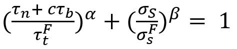 |
Equation 5 |
Here τn is the shear stress by normal load components, σS is the normal stress due to shear load component. And  ,
,  , c, α and β are coefficients.
This work included verification experiments of 42 kinds of homogenous steel stack-ups and 23 heterogeneous stack-ups. The strength levels of the steels used was between 270 MPa and 1500 MPa, and thickness between 0.55 mm and 2.3 mm. These experiments were used to evaluate the model and compare the results to the Wung model.
Conclusions
Overall, this new model considers interaction between normal and bending components as they have the same loading direction and plane. The current developed model was compared with the Wung model described above and has shown better results with a desirable error, especially for asymmetric material and thickness.
RSW Parameter Guidelines
This article summarizes a paper entitled, “RSW of 22MnB5 at Overlaps with Gaps-Effects, Causes, and Countermeasures”, by J. Kaars, et al.K-12
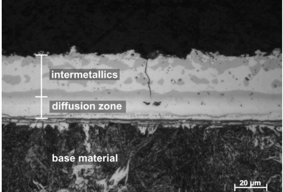
This study aims to elaborate on the influencing mechanisms of gaps on the welding result. Welding experiments at artificial gaps and finite element analysis (FEA) of the welding process have been used to investigate the matter. In both methods, the same configuration of two 1.5-mm-thick 22MnB5+AS150 welded with electrodes of the type ISO 5821 B0-16-20-40-6-30 was considered. Tensile tests yielded an ultimate tensile strength (UTS) of the press-hardened material of 1481 ± 53 MPa with a strain to fracture of 7.5 ± 0.26%. A microsection of the coating morphology after heat treatment can be found in Figure 1.
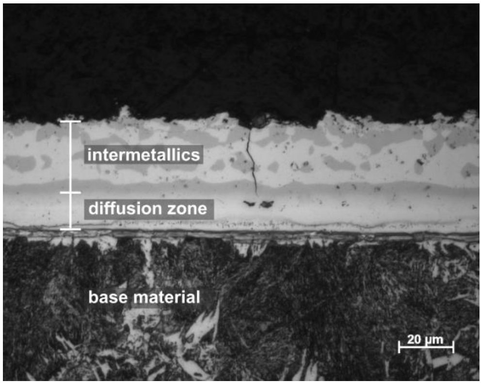
Figure 1: Morphology of the Aluminum-Silicon Coating.K-12
To set up an artificial and reproducible gap between the sheets, a dedicated fixture was used. It is displayed in Figure 2. All welding experiments were carried out with a 6-kN electrode force.
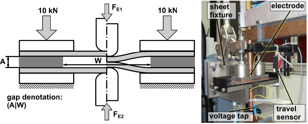
Figure 2: Fixture for Welding at Artificial Gaps, Definition of Quantities.K-12
In Table 1, the parameter variations of the gaps investigated in this work are presented.
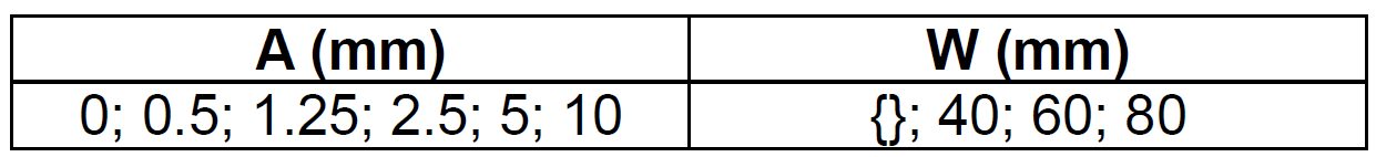
Table 1: List of Gap Parameters Investigated.K-12
A 7-kN maximum denting force was observed at the gap (10|60). With a gap of (10|40) the gap could not be closed with the machines’ 8-kN clamping force capacity. In comparative tests on mild steel for deep drawing a clamping force of about 2 kN was required to overcome the gap (10|60) (see Figure 3). The main effects diagram of the denting force clearly shows that the average denting force gets smaller with increasing support width and becomes larger with increasing gap clearance.
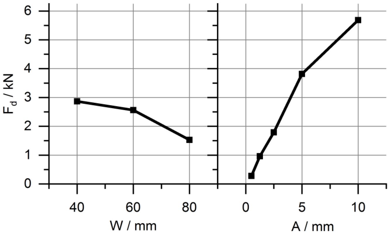
Figure 3: Main Effects Diagram of the Denting Force.K-12
In Figure 4, the achieved nugget diameters at different gaps using a constant machine setting of Iw,f = 6.4 kA are displayed.
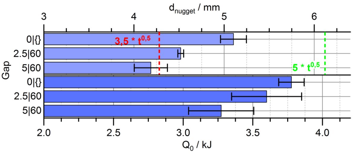
Figure 4: Effect of Gaps on Nugget Diameter, Absolute and Relative Results.K-12
A two-staged welding program, starting with a preheat current followed by a larger finishing current proved to yield the best welding results with the material used, cf., Figure 5. In Figure 5, the applied welding current program along with the measured and computed total resistance curve is displayed.
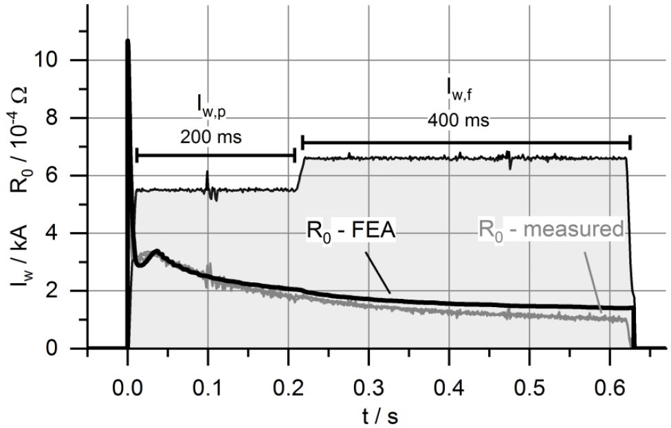
Figure 5: Exemplary Total Resistance Curve of a Weld without Gap, Measured and Computed Results.K-12
The FEA model can represent the welding process in terms of nugget diameter, dynamic resistance curve, and total electric energy with great accuracy. In Figure 6, the partial resistances of the weld as computed by FEA are composed.
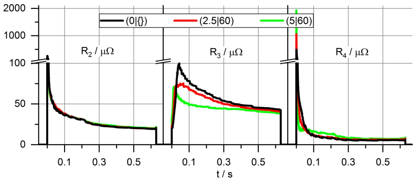
Figure 6: Partial Electrical Resistances at Different Gap Configurations.K-12
In the top section of Figure 7, the computed sheet thickness curve during the process for different gaps is presented. Increased electrode indentation during welding at gaps is the reason for reduced resistance and, therefore, results in reduced nugget diameters. The lower section of Figure 7 shows the plastic strains in the sheets along with a visibly reduced sheet thickness.
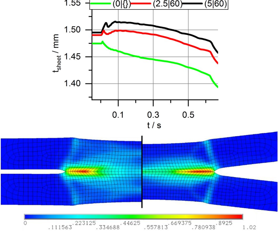
Figure 7: Dynamic Sheet Thickness (up) and Plastic Strain in millimeters at Different Gaps (low, to scale).K-12
Additional welding experiments were performed to clarify, if increased welding current can counter the gap effect and maintain the energy level of the weld. The results are shown in Figure 8. They prove that increased weld current is sufficient to not only maintain the nugget diameter at gaps, but moreover increase it.
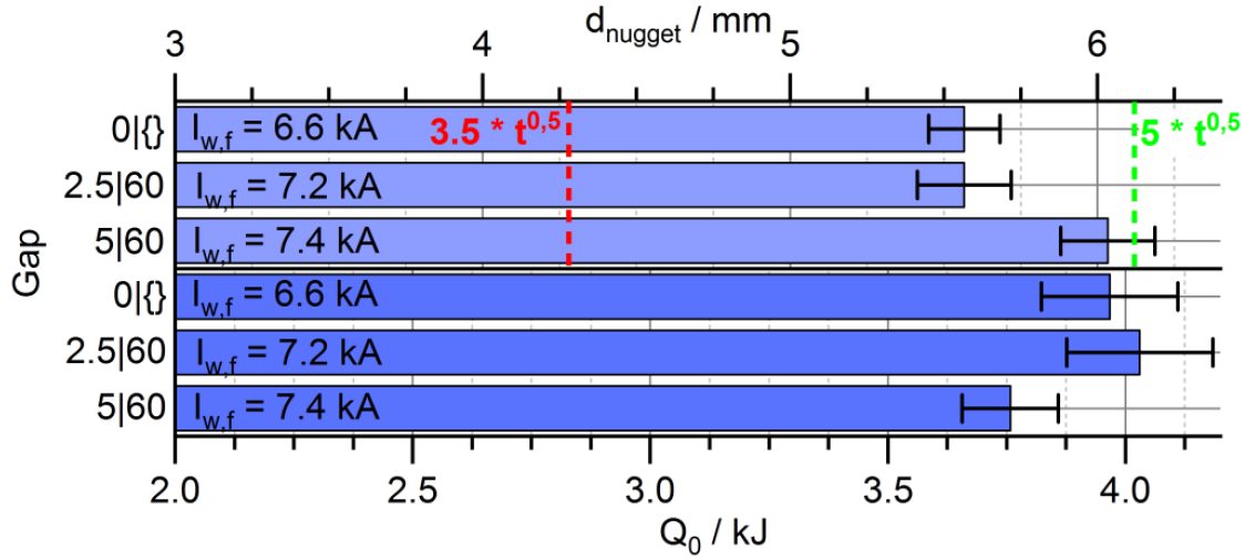
Figure 8: Nugget Diameter and Energy of Spot Welds near the Splash Limit at Overlaps with Gap.K-12
Results of further investigations on the weldability lobe of the joint are composed in Figure 9.. It is visible that with increasing gap the current range shifts toward larger currents and gets narrower.
RSW Joint Performance Testing
This articles summarizes a paper entitled, “New Test to Analyze Hydrogen Induced Cracking Susceptibility in Resistance Spot Welds,” by M. Duffey.D-10
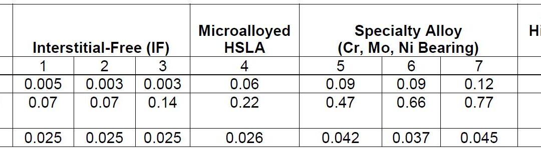
This study aims to develop a new weldability test to analyze the susceptibility of HIC in RSW of different steels. A total of eight different steel samples were analyzed with their carbon content, associated American Welding Society (AWS) carbon equivalencies, and gauges shown in Table 1. All materials were tested in the full-hard condition (all have been cold-rolled).
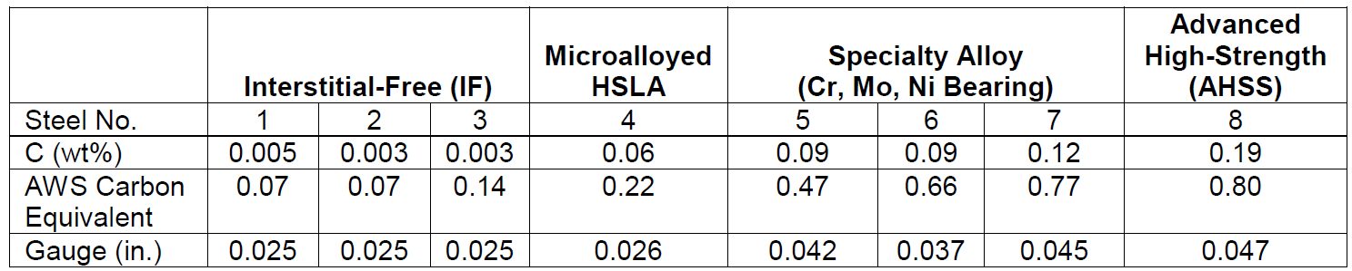
Table 1: Tested Steels, Carbon Equivalencies, and Steel Gauge.D-10
The associated parameter ranges for welds made with each steel are in Table 2. The resistance spot weld was made in the middle of the sheets, as shown in the test setup in Figure 1. There was a total of 18 test samples (nine not painted and wiped, nine painted) for each material tested.
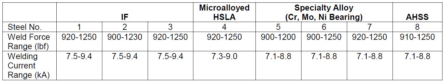
Table 2: Welding Parameters.D-10
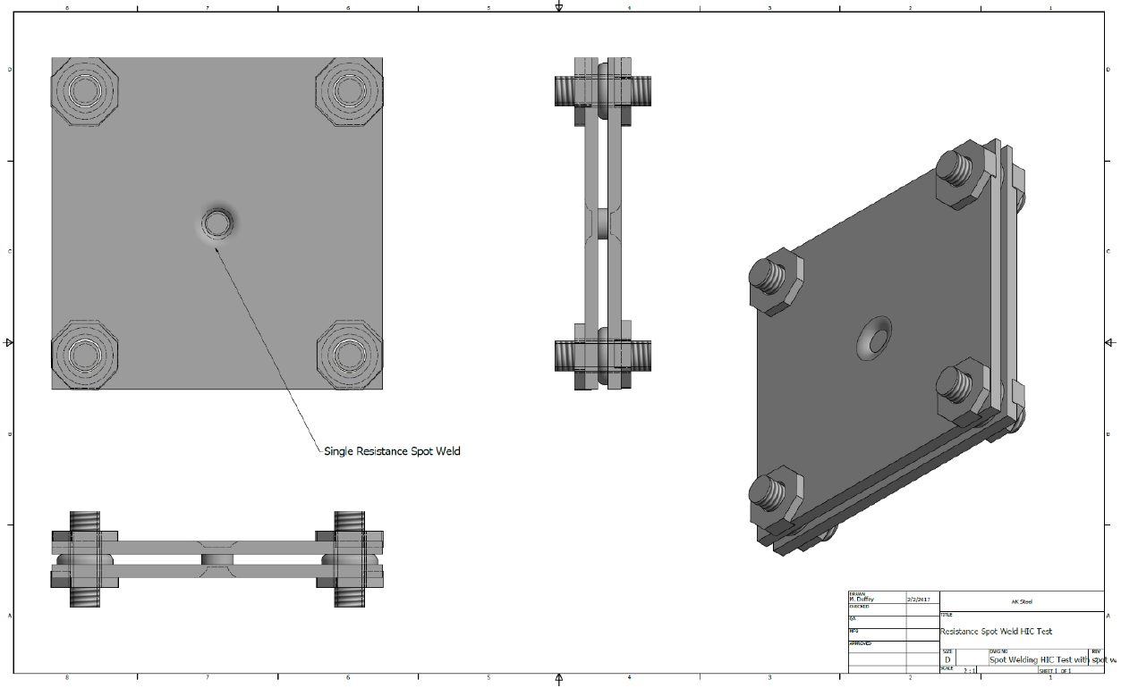
Figure 1: HIC Test for Resistance Spot Welds Schematic.D-10
Figure 2A shows the results of the 3- × 3-in. tests. Figure 2B shows the results of the 4- × 4-in. tests. Figure 2C shows the results of the 5- × 5-in. tests.
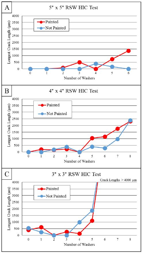
Figure 2: Results of the Three Different Test Sizes on AHSS.D-10
Cracks consistently initiated at the periphery of the weld nugget where the two steel sheets came together. Cracks then propagated either in the weld metal or HAZ, as shown in Figures 3 and 4.
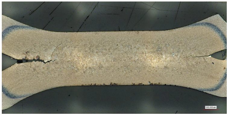
Figure 3: Cracking in the Weld Metal of Steel 8.D-10
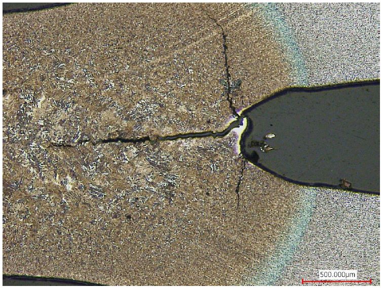
Figure 4: Cracking in Both the Weld Nugget and HAZ in Steel 8.D-10
Figure 5 displays the results from Steels 1, 4, and 5. Steel 1 is the most resistant (of the three) to HIC. For the three steels shown in Figure 5, the crack length (at each gap spacing) was longer for the painted sample than the non-painted sample.
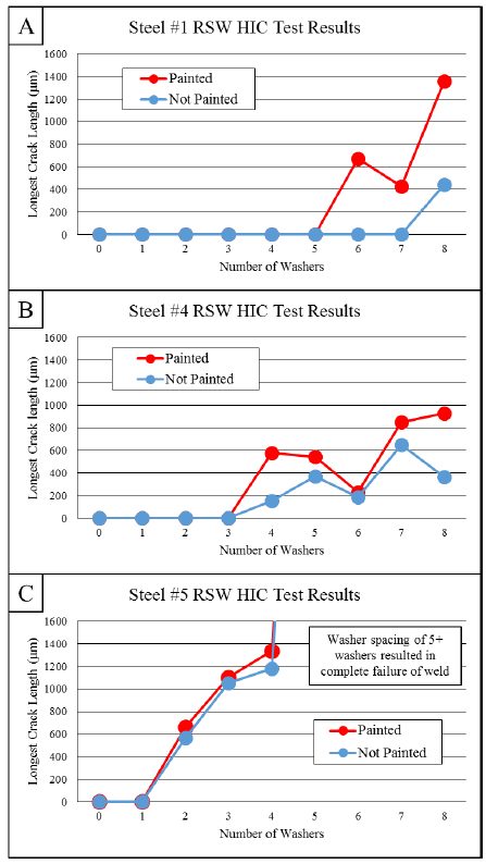
Figure 5. Test Results for Steels 1, 4, and 5.D-10
The microstructure of IF Steels 1-3 (Figure 6A) was ferrite. The microstructure of the high-strength low-alloy (HSLA) Steel 4 (Figure 6B) was a mixture of grain boundary ferrite, martensite, and possibly some bainite. The microstructure of the specialty alloy Steels 5-7 and AHSS Steel 8 (Figure 6C) was entirely martensite.
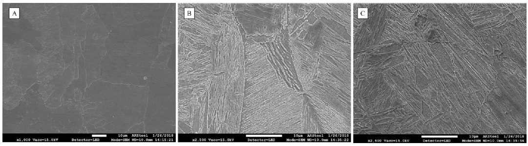
Figure 6: Microstructures of the Different Weld Nuggets.D-10
Figure 7 shows the fracture surface of a crack completely through Steel 7.
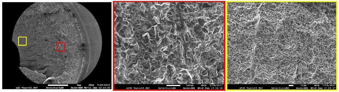
Figure 7: Fracture Surface of Cracked Weld in Steel 7.D-10
The average and maximum hardness results of spot welds in each material are summarized in Figure 8.
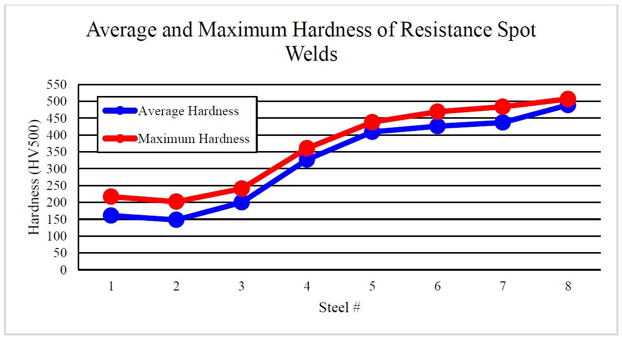
Figure 8. The Average and Maximum Hardness of HAZ and Weld Nugget in Resistance Spot Welds of Each Steel.D-10
Figure 9 is a graph that displays the carbon equivalence, number of washers where cracking first began, and average hardness of the weld nugget and HAZ in each steel.
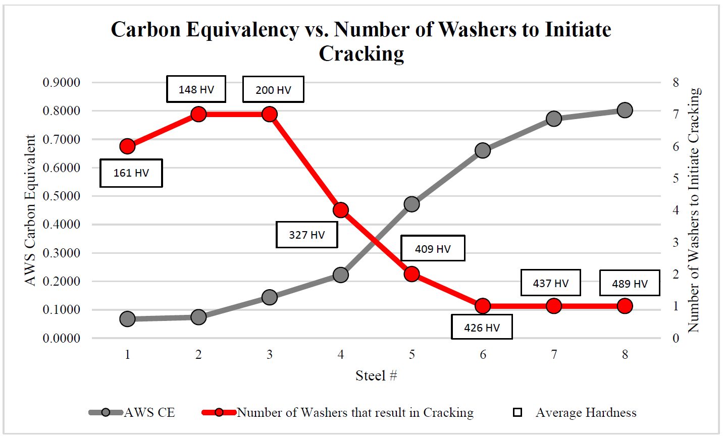
Figure 9: Carbon Equivalency vs. Number of Washers to Initiate Cracking.D-10
Resistance Spot Welding
This article summarizes a paper entitled, “High Strength Steel Spot Weld Strength Improvement through in situ Post Weld Heat Treatment (PWHT)”, by I. Diallo, et al.D-9
The study proposes optimal process parameters and process robustness for any new spot welding configuration. These parameters include minimum quenching time, post weld time, and post-welding current.
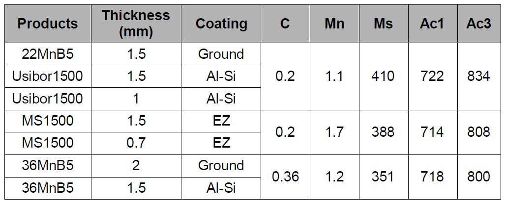
Three different chemical compositions are considered in this study and are listed in Table 1.
Table 1: Chemical composition and metallurgical data of products tested. Formulas used to calculate Ms, Ac1 and Ac3 are from “Andrews Empirical Formulae for the Calculation of Some Transformation Temperatures.”D-9
Welding configurations and process parameters are described in Table 2.
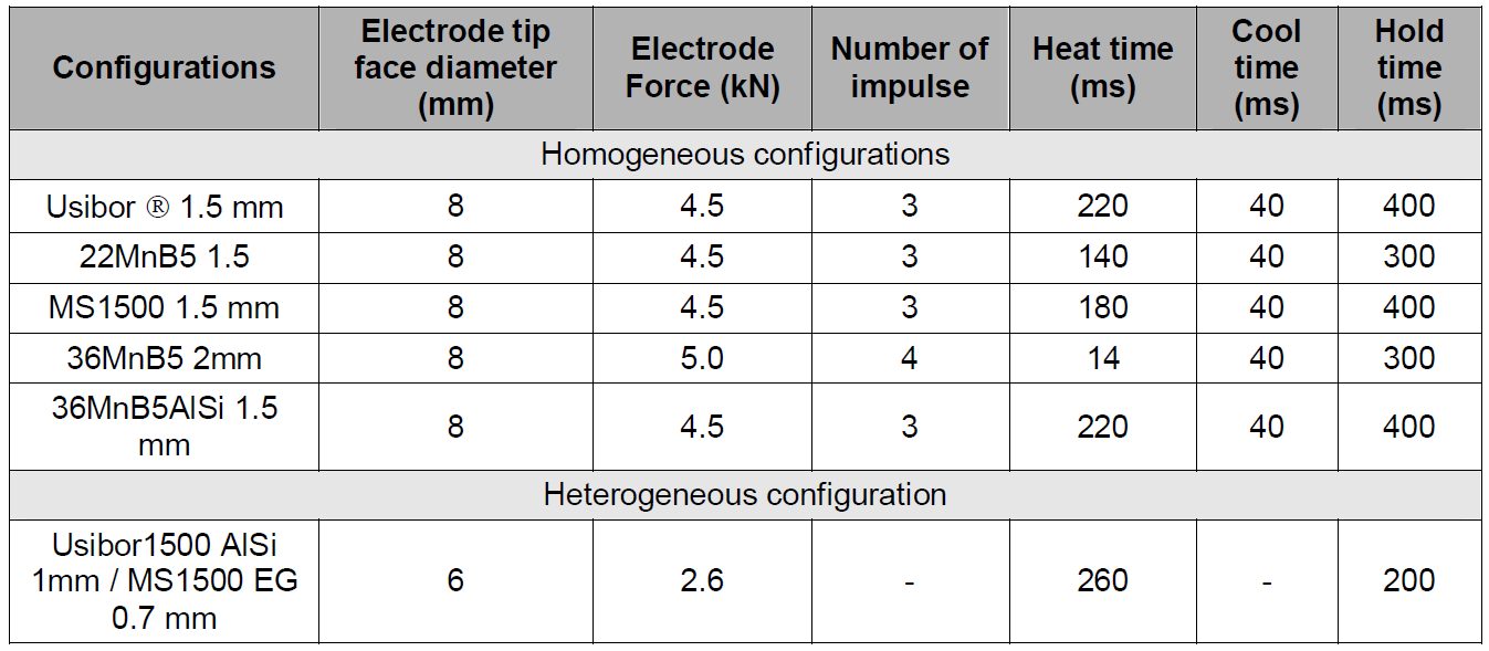
Table 2: Welded configurations and welding parameters used in reference cases.D-9
Cross Tensile Strength for MS1500EG 1.5 mm homogenous configuration is seen in Figure 1. Table 3 lists the reference data for the other configurations in this study.
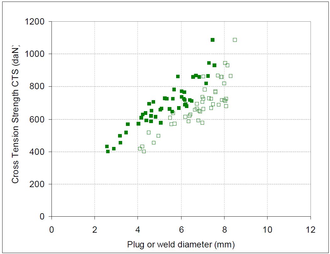
Figure 1: Cross Tensile Strength for MS1500EG 1.5 mm homogenous configuration as a function of plug (closed symbols) or weld (open symbols) diameter.D-9
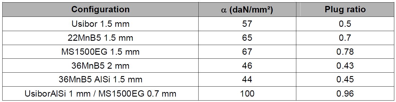
Table 3: Average α and plug ratio along the welding range for reference configurations.D-9
Figure 2 and 3 depict micrographs of welds after PWHT applied on 36MnB5 2 mm homogeneous configuration. These micrographs illustrate the evolution of the microstructure during PWHT and are labeled accordingly. Figure 4 shows the microhardness profiles in the welds described in Figure 3. It is clear that the Mf temperature was reached in the entire weld before application of PWHT.
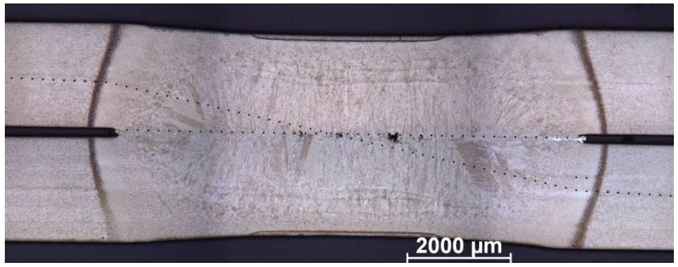
Figure 2: Micrograph of reference weld for 36MnB5 2mm homogeneous configuration.D-9
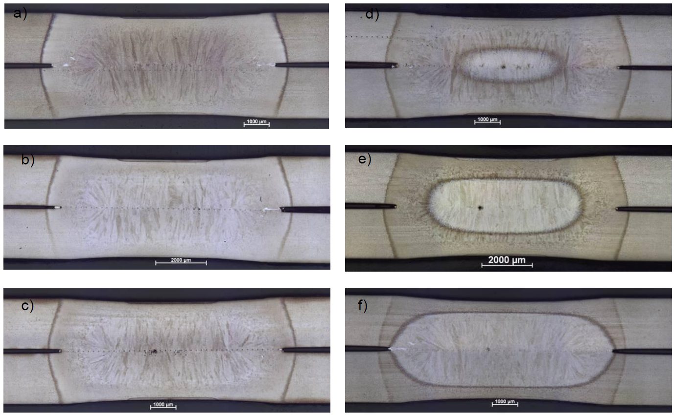
Figure 3: Micrographs of welds after post weld heat treatment applied on 36MnB5 2 mm homogeneous configuration with 70 periods of quenching and post welding current of a) 54%Iw, b) 62%Iw, c) 65% d) 67%Iw, e) 71%Iw and f ) 78%Iw.D-9
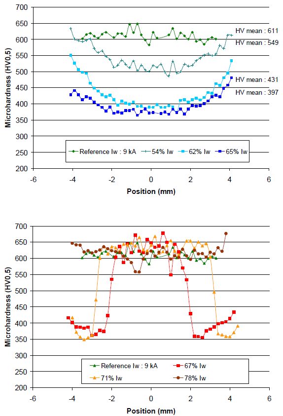
Figure 4: Microhardness profiles in welds after post weld treatment applied on 36MnB5 2mm homogeneous configuration with 70 periods of quenching ; these measurements correspond to micrographs shown in Figure 2 and Figure 3.D-9
Similar methodology was performed on partial quenching examples with AISI coating and electrogalvanized coating. Table 4 lists the minimum quenching times that were determined experimentally for each configuration.
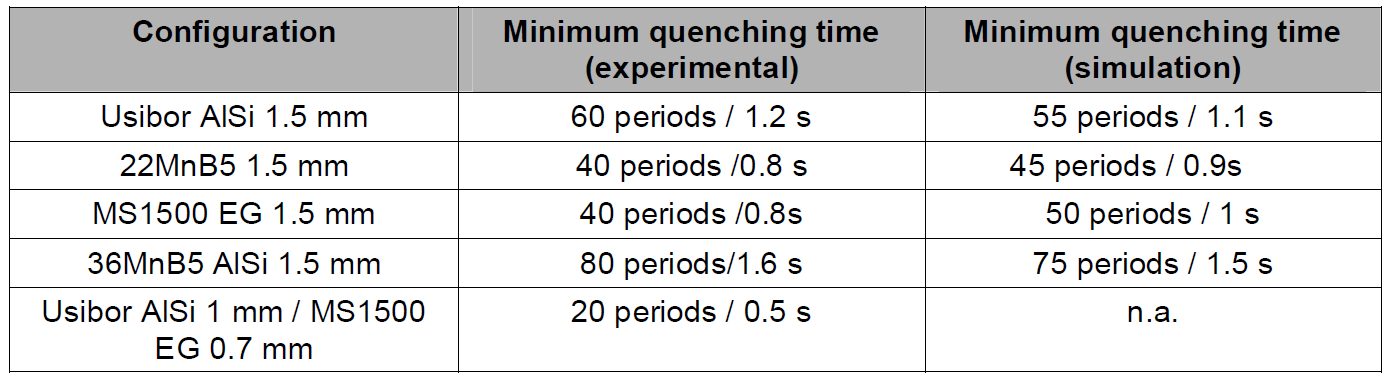
Table 4: Minimum quenching times determined experimentally and through Sorpas simulation.D-9
For selection of post weld time, a slightly different methodology was performed. Optimal quenching time was determined and used to construct the evolution of post weld current range as a function of post weld time as described in Figure 5. This figure shows that post welding current range is stable between 60 and 30 periods of post weld time.
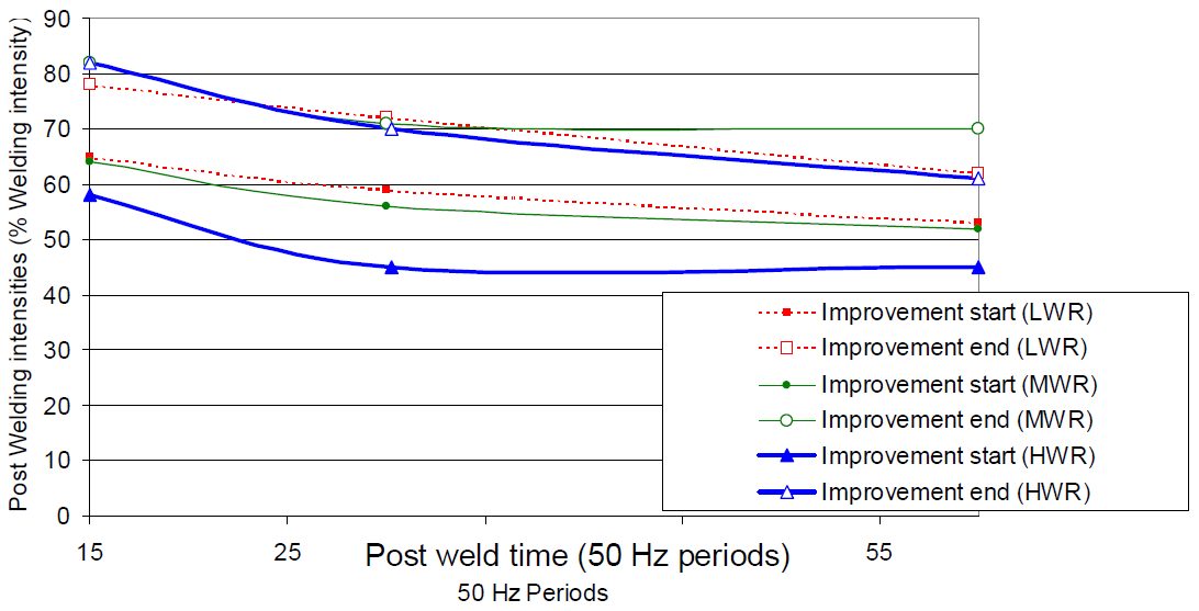
Figure 5: Evolution of post welding current range as a function of post weld time for three welding current levels.D-9
Notch tip hardness measured after different post welding currents has been reported in Figure 6. From this result, a notch tip tempering range is found to be between 400 °C and Ac1.
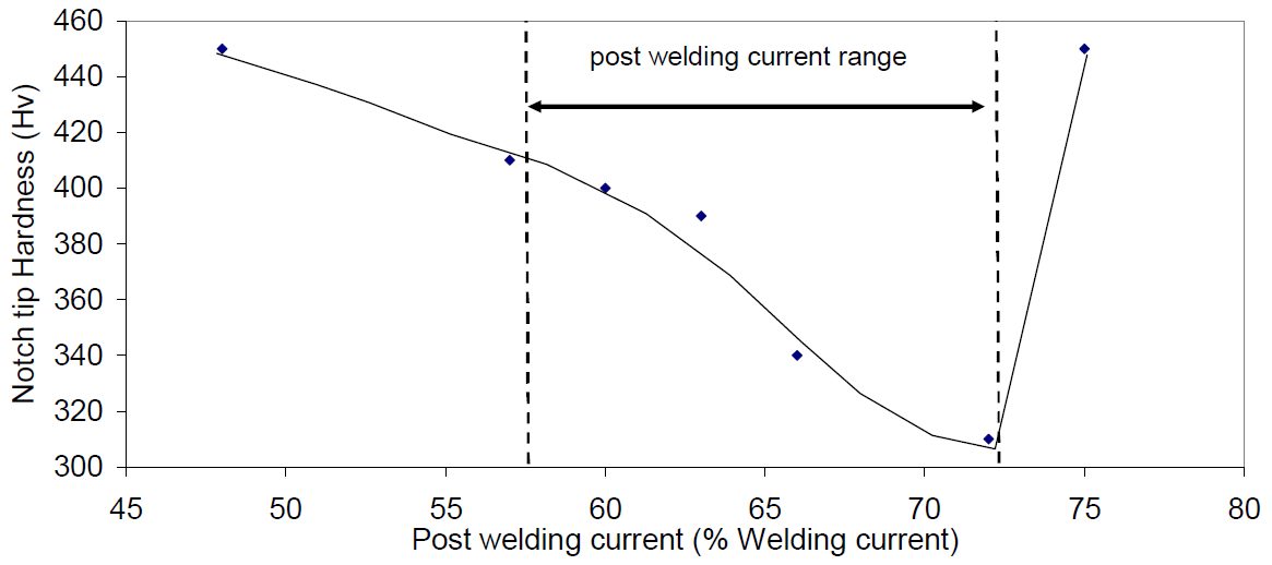
Figure 6: Relationship between measured notch tip hardness and post-welding current (Usibor1500 AlSi 1.5mm, LWR).D-9
Using the notch tip tempering range, a post welding current range can be calculated from Sorpas calculations in Figure 7.
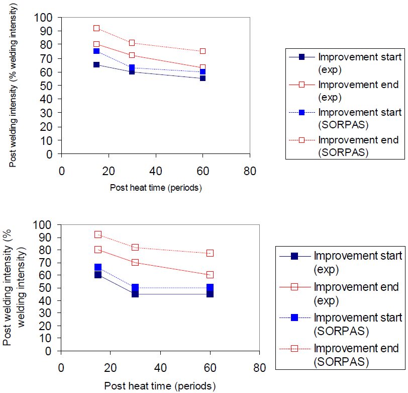
Figure 7: Experimental and numerical post welding current ranges for Usibor1500 AlSi 1.5 mm configuration (above: LWR, below: HWR).D-9
Results are displayed in Figure 8 for post weld time for MS1500 EZ with low welding current LWR.
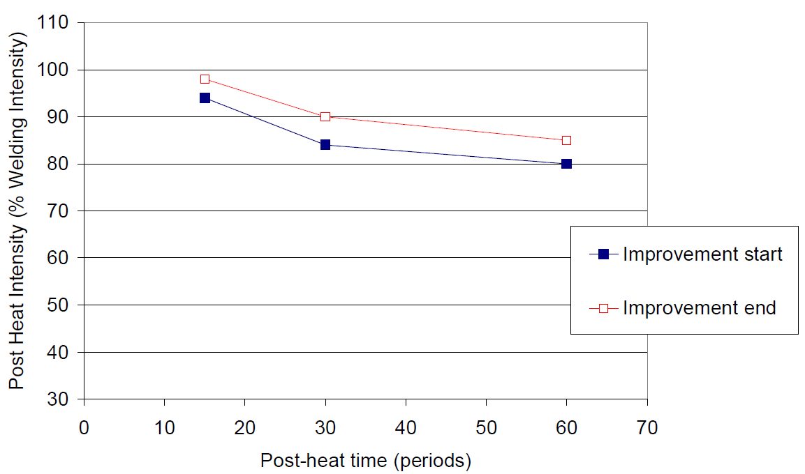
Figure 8: Evolution of post welding current ranges for different post welding times in LWR.D-9
Figure 9 displays results for MS1500 EG 1.5mm configuration.
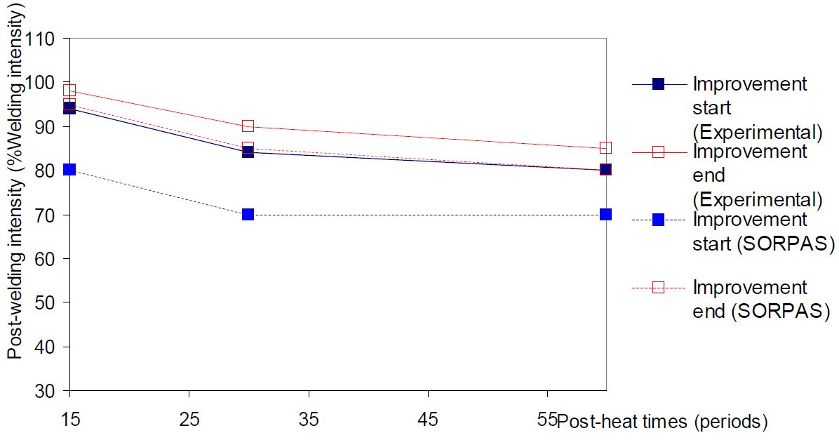
Figure 9: MS1500 EG 1.5 mm configuration experimental and simulated post welding current ranges (LWR).D-9
The same methodology was applied to other configurations and the results are displayed in Table 5.
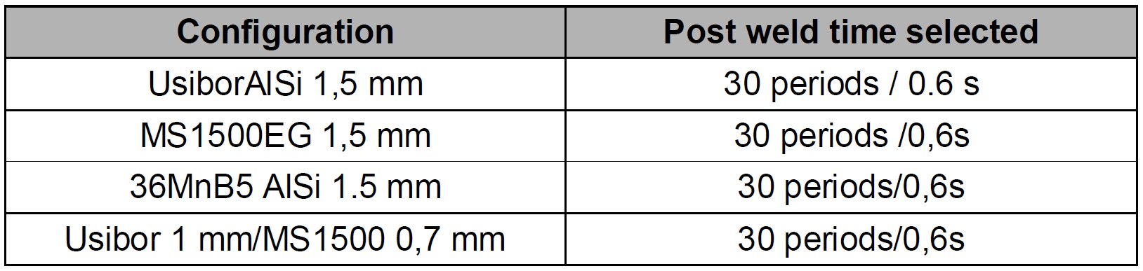
Table 5: Post weld times selected.D-9
Interpolation between experiments was carried out to create a robustness and performance tempering map that is displayed in Figure 10. The map shows tremendous improvement of cross tension strength can be achieved through PWHT. Additionally, the optimal post welding current is around 65% of welding current, and the CTS level reached for LWR and HWR without PWHT is very similar.
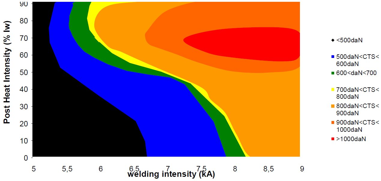
Figure 10: Tempering map for Usibor ® AlSi 1.5 mm homogeneous configuration, drawn after experimental results shown on Figure 9.D-9
Figure 11 displays cross-tension results for Usibor1500 AlSi using the optimized cycle [Metallurgical Post Weld Heat Treatment (MPWHT)].
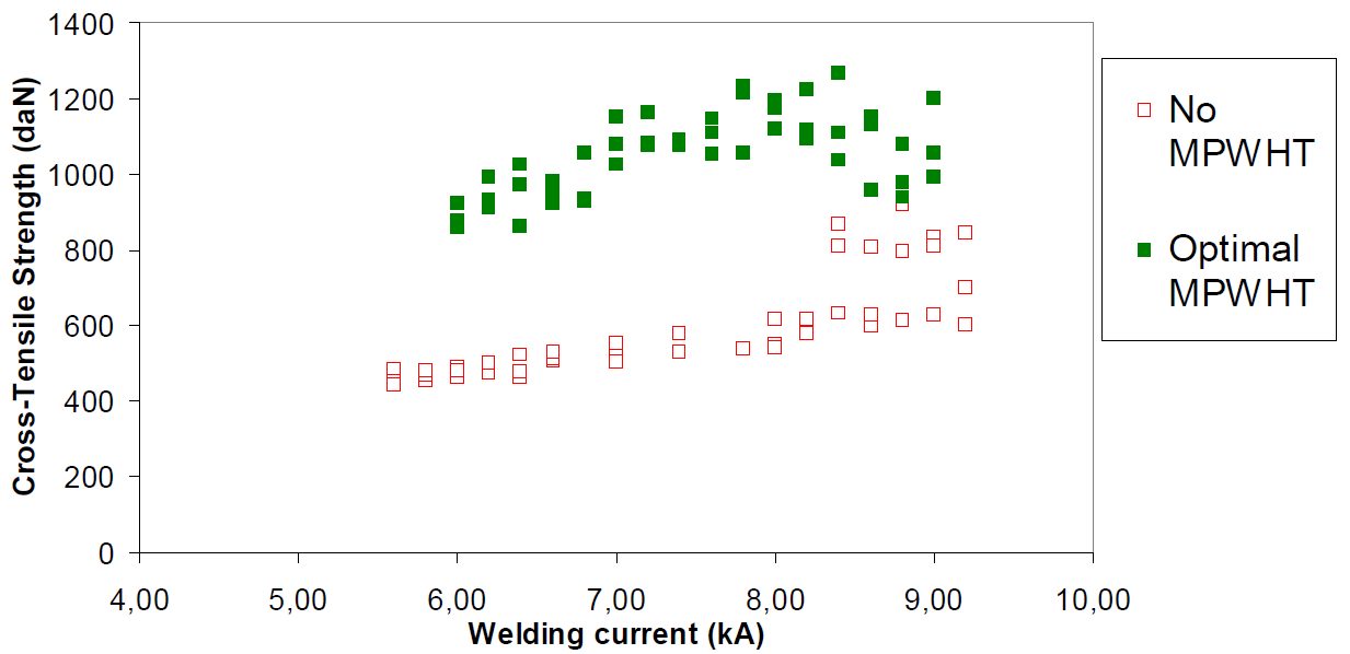
Figure 11: Comparison of CTS along the welding current range, with and without MPWHT.D-9
Table 6 and Figure 12 display all the reference and MPWHT spot weld performance after Cross-Tension testing.
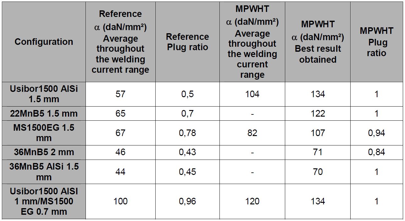
Table 6: ɑ coefficients and plug ratios for reference and with post treatment for all the configurations.D-9
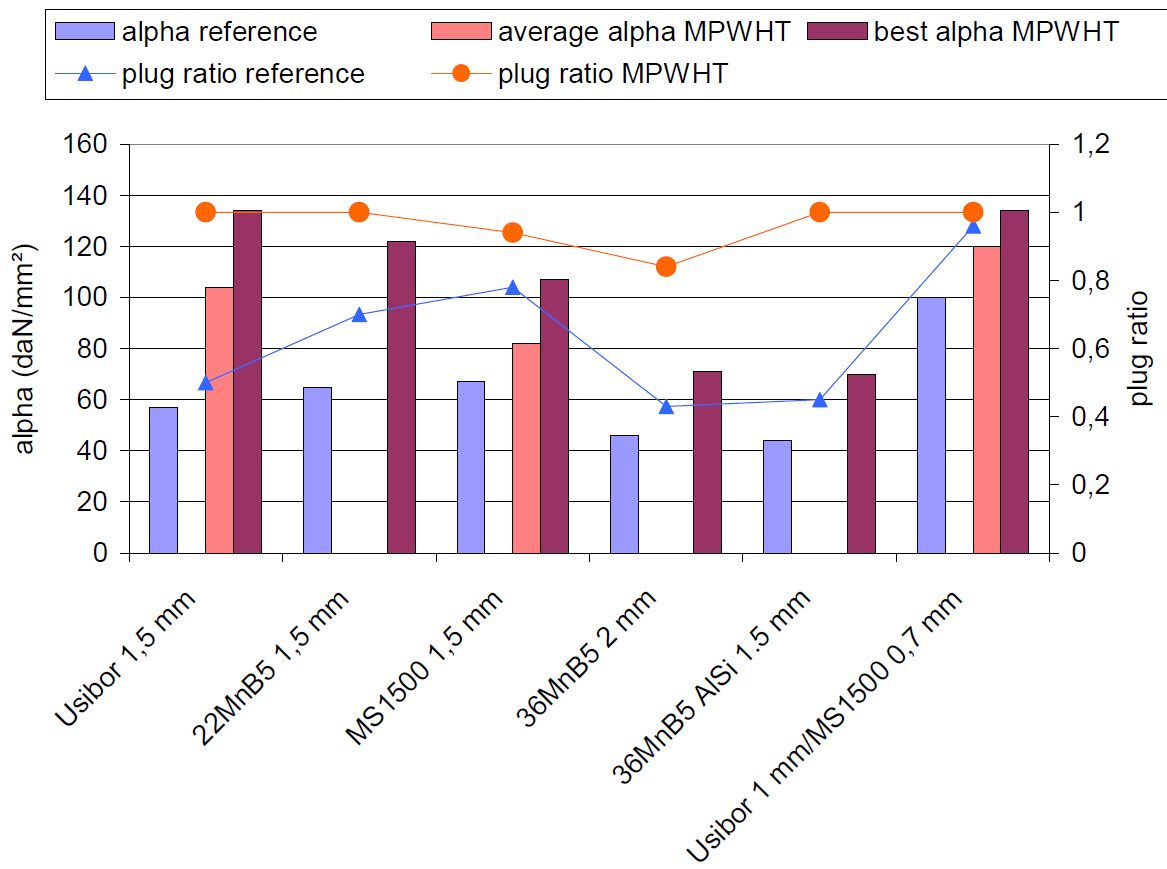
Figure 12: ɑ coefficients and plug ratios for reference and with post treatment for all the configurations.D-9
MPWHT, aiming at tempering the martensite formed during spot welding of Advanced High-Strength Steels, has been studied for several configurations both experimentally and numerically. The methodology proposed in this study is available to determine the optimal process parameters and the process robustness for any new configuration. Among the major results brought by this study:
- A minimum quenching time is necessary to fully transform the weld into martensite before post weld heat treatment; this time can be determined based on metallographic observations, and depends strongly on sheets thickness, chemistry and coating.
- The post weld time is not very sensitive to the configuration welded; 0.6 s seems a reasonable time, although it may be reduced further.
- The post welding current can be simply expressed as a percentage of the welding current, the efficient level being then constant along the welding current range.
- A range of post welding currents can be determined, allowing an efficiency of the post weld heat treatment process. Tempering maps allow common visualization of the welding current and post welding current ranges in two dimensions, to characterize the whole process robustness.
- MPWHT is very efficient in improving the mechanical weld performance in opening mode; cross-tension strength can be doubled in some cases; the process efficiency depends on the chemistry of the grades.
- In case of heterogeneous configuration, the so-called “positive deviation” can give a good performance to the weld even without MPWHT, limiting the improvement brought after post treatment.
RSW of Dissimilar Steel
This article summarizes a paper entitled, “Higher than Expected Strengths from Dissimilar Configuration Advanced High-Strength Steel Spot Welds”, by E. Biro, et al.B-6
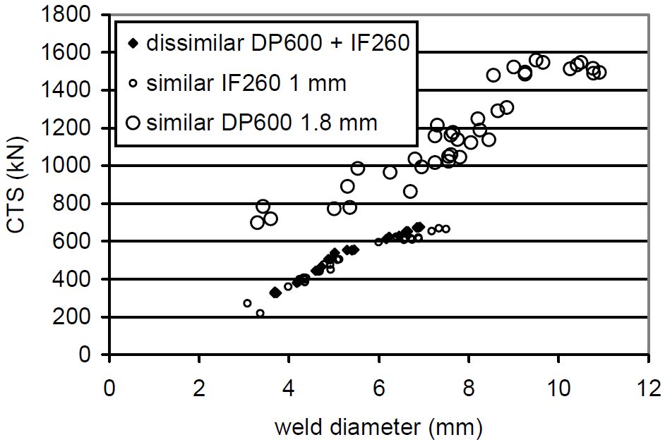
This study shows that the cross tension strength (CTS) is always higher than the strength expected from the lower strength material in the joint. Figure 1 verifies the assumption that the load bearing capacity of a heterogeneous configuration is supposed to equal the minimum strength of both homogenous assemblies. Material used in this study was a 1 mm low carbon equivalent Dual Phase 980 (DP980 LCE) steel.
Figure 1: Example of dissimilar configuration with CTS matching the “minimum rule”.B-6
The materials chosen for this study are in Table 1.
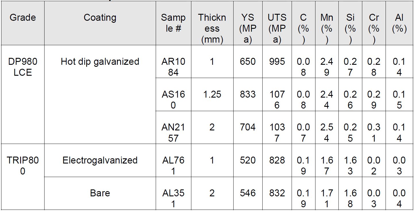
Table 1: Steel sheet samples.B-6
The material thickness combinations for all of the two sheet joints are shown in Table 2.
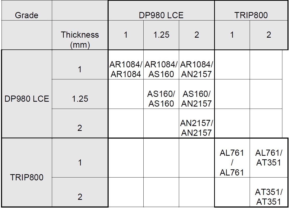
Table 2: Welded 2-sheet configurations.B-6
The three-sheet stackups all were made using the 1 mm DP980 LCE. These configurations were designed to understand what happens in such cases, knowing that three-sheet welding is very common in car body manufacturing. The three-sheet stackup configurations are shown in Figure 2 and are as were follows:
- a square DP980 coupon (patch) is inserted between the two classical cross-tension coupons for welding (1+patch+1 mm);
- two coupons oriented the same way welded with one coupon oriented in the transverse direction to form a cross-tension sample (1+[1+1] mm);
- same configuration as a) but the external coupon is removed by manual torsion before cross-tension testing (1+1+0 mm);
- same configuration as a), but the two coupons oriented the same way are first spot welded together strongly (with several spots) in the extremities, before the actual 3-sheet spot weld is done ([1++++1]+1 mm).
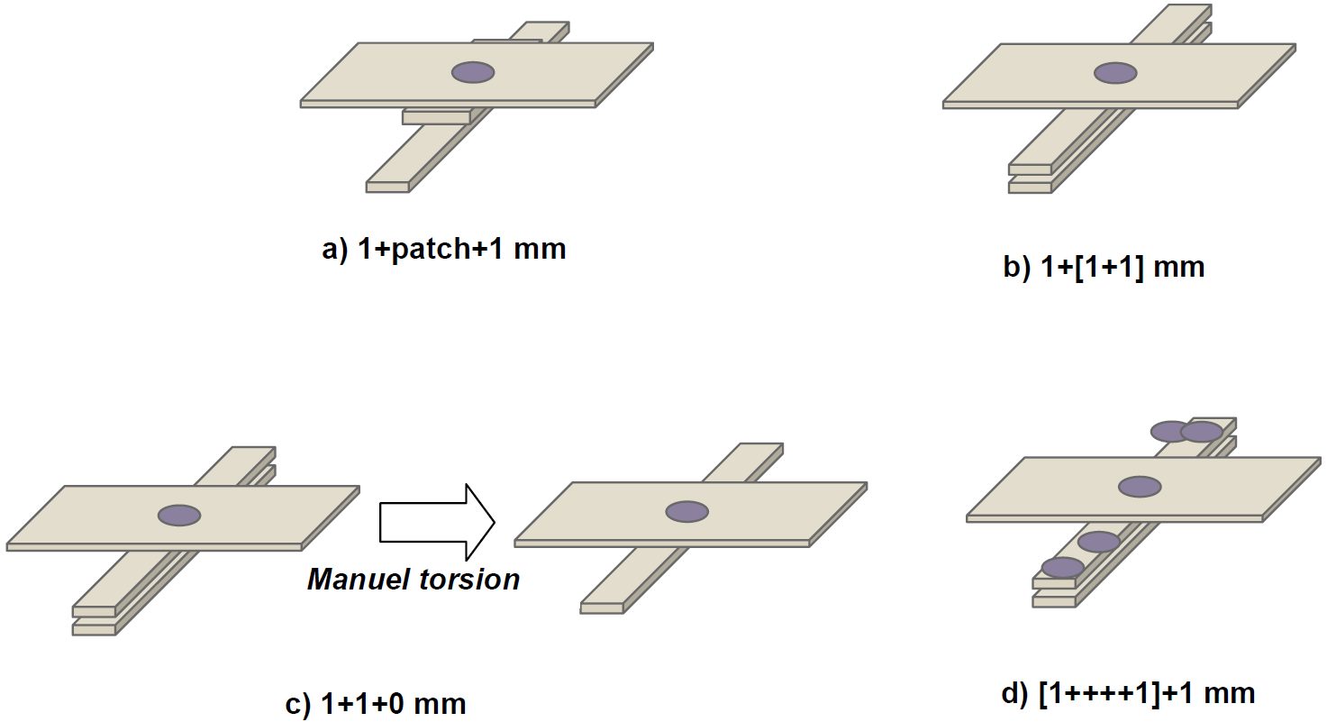
Figure 2: Three-sheet configurations based on 1mm DP980 LCE sample.B-6
The welding parameters for each configuration are listed in Table 3.
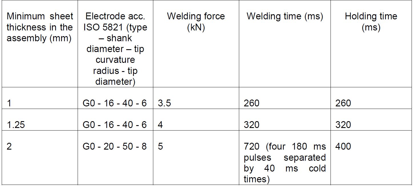
Table 3 : Welding parameters.B-6
CTS is strongly dependent on weld diameter (Figure 3).
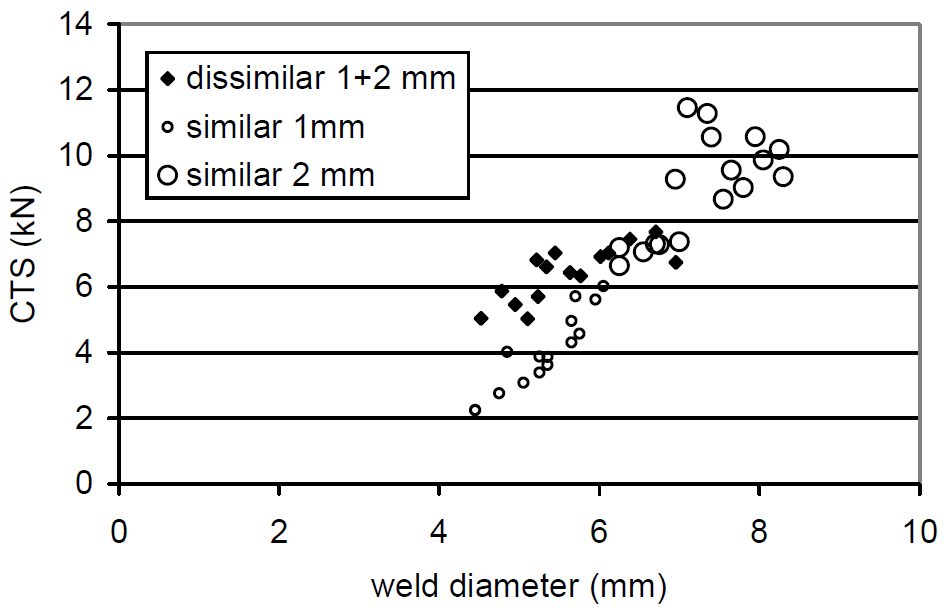
Figure 3: Cross-tension Strength for TRIP800 configurations.B-6
CTS for the main DP980 configurations are shown as a function of weld diameter in Figures 4 and 5.
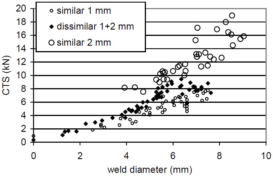
Figure 4: Cross-tension Strength for DP980 1+1, 1+2 and 2+2 configurations.B-6
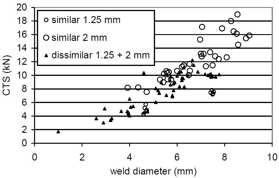
Figure 5: Cross-tension Strength for DP980 1.25+1.25, 1.25+2 and 2+2 configurations.B-6
The three-sheet configurations based on 1mm DP980 LC results are shown in Figures 6 and 7. These results again verify that dissimilar configuration performances appear above the “minimum rule” assumption described in Figure 1.
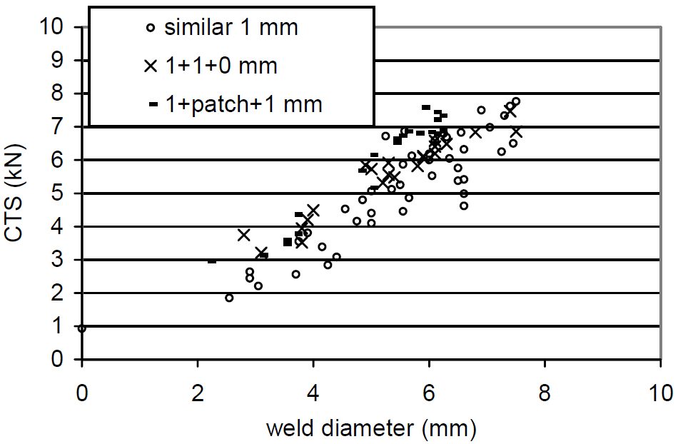
Figure 6: Cross-tension Strength for DP980 1+1, 1+1+0 and 1+patch+1 configurations.B-6
![Figure 7: Cross-tension Strength for DP980 1+1, 1+2, 1+[1+1]and [1+++1]+1 configurations.](https://ahssinsights.org/wp-content/uploads/2020/07/3114c_Fig7.jpg)
Figure 7: Cross-tension Strength for DP980 1+1, 1+2, 1+[1+1]and [1+++1]+1 configurations.B-6
The observation that CTS is greater than predicted by the “minimum rule” has been called a “positive deviation” from the expected strengths.
This work concluded that while material qualification tests are frequently based on similar welding configurations, real car body applications are quite systematically dissimilar configurations. For spot welds failing in plug mode, the strength of the assembly only depends on the weakest material strength. In case of AHSS+AHSS welded combinations, however, things turn out to be different. Similar grade but dissimilar thickness High-Strength Steel configurations have been spot welded and tested in Cross-Tension. The following main conclusions can be highlighted:
- For dissimilar thickness configurations, the cross-tensile strength is above the standard “minimum rule” assumptions, this phenomenon being called a “positive deviation”;
- Limited thermal and notch location effects can explain part of this positive deviation, but the main reason is mechanical;
- As evidenced through several analytic and numerical studies, this mechanical effect is due to the less severe local stresses at the notch in case of uneven thickness, and improves the positive deviation when the thickness ratio increases. Although widely used for material qualification and scientific purposes, similar configurations appear as the worst case in terms of cross-tension performance for high strength steels. Actual vehicle design should consider positive deviation in dissimilar configurations to maximize the potential strength of spot welds in High-Strength steels.