RSW Masterclass
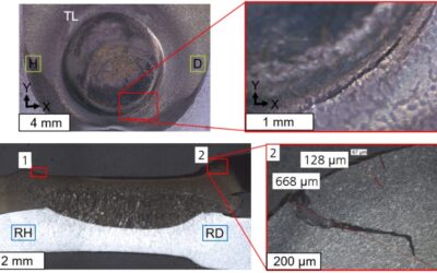
Four Steps to Mitigate Liquid Metal Embrittlement When Welding Steel
Liquid Metal Embrittlement (LME) during Resistance Spot Welding (RSW) can cause cracks when welding advanced high strength steels. Recent advances in steel metallurgy, resistance spot welding processing and accompanying simulation tools have substantially improved the...
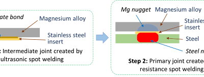
Resistance Spot Welding AHSS to Magnesium
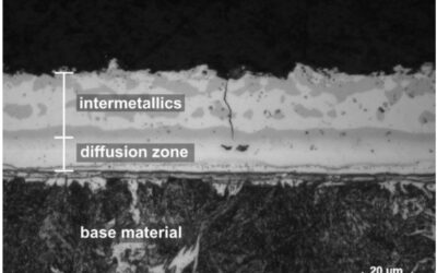
This blog is a short summary of a published comprehensive research work titled: "Peculiar Roles of Nickel Diffusion in Intermetallic Compound Formation at the Dissimilar Metal Interface of Magnesium to Steel Spot Welds" Authored by Luke Walker, Carolin Fink,...
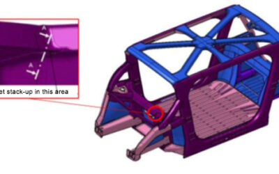
Resistance Spot Welding: 5T Dissimilar Steel Stack-ups for Automotive Applications
Urbanization and waning interest in vehicle ownership point to new transport opportunities in megacities around the world. Mobility as a Service (MaaS) – characterized by autonomous, ride-sharing-friendly EVs – can be the comfortable, economical, sustainable transport...
LME Simulation during RSW
Modern car bodies today are made of increasing volumes of Advanced High-Strength Steels (AHSS), the superb performance of which facilitates lightweighting concepts (see Figure 1). To join the different parts of a car body and create the crash structure, the components...

Modelling RSW of AHSS
Modelling resistance spot welding can help to understand the process and drive innovation by asking the right questions and giving new viewpoints outside of limited experimental trials. The models can calculate industrial-scale automotive assemblies and allow...
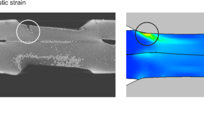
RSW Failure Prediction
This article summarizes the findings of a paper entitled, "Prediction of Spot Weld Failure in Automotive Steels,"L-48 authored by J. H. Lim and J.W. Ha, POSCO, as presented at the 12th European LS-DYNA Conference, Koblenz, 2019. To better predict car crashworthiness...
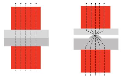
Projection Welding
As with resistance spot welding in automotive applications, projection welding also is used to join two overlapping sheets of relatively thin metal. The process involves pressing a projection or number of projections in one of the plates and welding the two plates...
RSW of 22MnB5 at Overlaps
This article summarizes a paper entitled, "RSW of 22MnB5 at Overlaps with Gaps-Effects, Causes, and Countermeasures", by J. Kaars, et al.K-12 This study aims to elaborate on the influencing mechanisms of gaps on the welding result. Welding experiments at artificial...