![Considerations When Deciding Whether to Cold Form or Hot Form]()
Automakers contemplating whether a part is cold stamped or hot formed must consider numerous ramifications impacting multiple departments. The considerations below relative to cold stamping are applicable to any forming operation occurring at room temperature such as roll forming, hydroforming, or conventional stamping. Similarly, hot stamping refers to any set of operations using Press Hardening Steels (or Press Quenched Steels), including those that are roll formed or fluid-formed.
Equipment
There is a well-established infrastructure for cold stamping. New grades benefit from servo presses, especially for those grades where press force and press energy must be considered. Larger press beds may be necessary to accommodate larger parts. As long as these factors are considered, the existing infrastructure is likely sufficient.
Progressive-die presses have tonnage ratings commonly in the range of 630 to 1250 tons at relatively high stroke rates. Transfer presses, typically ranging from 800 to 2500 tons, operate at relatively lower stroke rates. Power requirements can vary between 75 kW (630 tons) to 350 kW (2500 tons). Recent transfer press installations of approximately 3000 tons capacity allow for processing of an expanded range of higher strength steels.
Hot stamping requires a high-tonnage servo-driven press (approximately 1000 ton force capacity) with a 3 meter by 2 meter bolster, fed by either a roller-hearth furnace more than 30 m long or a multi-chamber furnace. Press hardened steels need to be heated to 900 °C for full austenitization in order to achieve a uniform consistent phase, and this contributes to energy requirements often exceeding 2 MW.
Integrating multiple functions into fewer parts leads to part consolidation. Accommodating large laser-welded parts such as combined front and rear door rings expands the need for even wider furnaces, higher-tonnage presses, and larger bolster dimensions.
Blanking of coils used in the PHS process occurs before the hardening step, so forces are low. Post-hardening trimming usually requires laser cutting, or possibly mechanical cutting if some processing was done to soften the areas of interest.
That contrasts with the blanking and trimming of high strength cold-forming grades. Except for the highest strength cold forming grades, both blanking and trimming tonnage requirements are sufficiently low that conventional mechanical cutting is used on the vast majority of parts. Cut edge quality and uniformity greatly impact the edge stretchability that may lead to unexpected fracture.
Responsibilities
Most cold stamped parts going into a given body-in-white are formed by a tier supplier. In contrast, some automakers create the vast majority of their hot stamped parts in-house, while others rely on their tier suppliers to provide hot stamped components. The number of qualified suppliers capable of producing hot stamped parts is markedly smaller than the number of cold stamping part suppliers.
Hot stamping is more complex than just adding heat to a cold stamping process. Suppliers of cold stamped parts are responsible for forming a dimensionally accurate part, assuming the steel supplier provides sheet metal with the required tensile properties achieved with a targeted microstructure.
Suppliers of hot stamped parts are also responsible for producing a dimensionally accurate part, but have additional responsibility for developing the microstructure and tensile properties of that part from a general steel chemistry typically described as 22MnB5.
Property Development
Independent of which company creates the hot formed part, appropriate quality assurance practices must be in place. With cold stamped parts, steel is produced to meet the minimum requirements for that grade, so routine property testing of the formed part is usually not performed. This is in contrast to hot stamped parts, where the local quench rate has a direct effect on tensile properties after forming. If any portion of the part is not quenched faster than the critical cooling rate, the targeted mechanical properties will not be met and part performance can be compromised. Many companies have a standard practice of testing multiple areas on samples pulled every run. It’s critical that these tested areas are representative of the entire part. For example, on the top of a hat-section profile where there is good contact between the punch and cavity, heat extraction is likely uniform and consistent. However, on the vertical sidewalls, getting sufficient contact between the sheet metal and the tooling is more challenging. As a result, the reduced heat extraction may limit the strengthening effect due to an insufficient quench rate.
Grade Options for Cold Stamped or Hot Formed Steel
There are two types of parts needed for vehicle safety cage applications: those with the highest strength that prevent intrusion, and those with some additional ductility that can help with energy absorption. Each of these types can be achieved via cold stamping or hot stamping.
When it comes to cold stamped parts, many grade options exist at 1000 MPa that also have decent ductility. The advent of the 3rd Generation Advanced High Strength Steels adds to the tally – the stress-strain curve of a 3ʳᵈ Gen QP980 steel is presented in Figure 1. Most of these top out at 1200 MPa, with some companies offering cold-formable Advanced High Strength Steels with 1400 or 1500 MPa tensile strength. The chemistry of AHSS grades is a function of the specific characteristics of each production mill, meaning that OEMs must exercise diligence when changing suppliers.

Figure 1: Stress-strain curve of industrially produced QP980.W-35
Martensitic grades from the steel mill have been in commercial production for many years, with minimum strength levels typically ranging from 900 MPa to 1470 MPa, depending on the grade. These products are typically destined for roll forming, except for possibly those at the lower strengths, due to limited ductility. Until recently, MS1470, a martensitic steel with 1470 MPa minimum tensile strength, was the highest strength cold formable option available. New offerings from global steelmakers now include MS1700, with a 1700 MPa minimum tensile strength, as well as MS 1470 with sufficient ductility to allow for cold stamping. Automakers have deployed these grades in cold stamped applications such as crossmembers and roof reinforcements, with some applications shown in Figure 2.

Figure 2: Cold-Stamped Martensitic Steel with 1500 MPa Tensile Strength used in the Nissan B-Segment Hatchback.K-57
Until these recent developments, hot stamping was the primary option to reach the highest strength levels in part shapes having even mild complexity. Under proper conditions, a chemistry of 22MnB5 could routinely reach a nominal or aim strength of 1500 MPa, which led to this grade being described as PHS1500, CR1500T-MB, or with similar nomenclature. Note that in this terminology, 1500 MPa nominal strength typically corresponds to a minimum strength of 1300 MPa.
The 22MnB5 chemistry is globally available, but the coating approaches discussed below may be company-specific.
Newer PHS options with a modified chemistry and subsequent processing differences can reach nominal strength levels of 2000 MPa. Other options are available with additional ductility at strength levels of 1000 MPa or 1200 MPa. A special class called Press Quenched Steels have even higher ductility with strength as low as 450 MPa.
The spectrum of grades available for cold-stamped and hot formed steel parts allows automakers to fine-tune the crash energy management features within a body structure, contributing to steel’s “infinite tune-ability” capability which gives automotive engineers design flexibility and freedoms not available from other structural materials.
Corrosion Protection
Uncoated versions of a grade must take a different chemistry approach than the hot dip galvanized (GI) or hot dipped galvannealed (HDGA) versions since the hot dip galvanizing process (Figure 3) acts as a heat treatment cycle that changes the properties of the base steel. Steelmakers adjust the base steel chemistry to account for this heat treatment to ensure the resultant properties fall within the grade requirements.

Figure 3: Schematic of a typical hot-dipped galvanizing line with galvanneal capability.
This strategy has limitations as it relates to grades with increasing amounts of martensite in the microstructure. Complex thermal cycles are needed to produce the highly engineered microstructures seen in advanced steels. Above a certain strength level, it is not possible to create a GI or HDGA version of that grade.
For example, when discussing fully martensitic grades from the steel mill, hot dip galvanizing is not an option. If a martensitic grade needs corrosion protection, then electrogalvanizing (Figure 4) is the common approach since an EG coating is applied at ambient temperature, which is low enough to avoid negatively impacting the properties. Automakers might choose to forgo a galvanized coating if the intended application is in a dry area that is not exposed to road salt.

Figure 4: Schematic of an electrogalvanizing line.
For press hardening steels, coatings serve multiple purposes. Without a coating, uncoated steels will oxidize in the austenitizing furnace and develop scale on the surface. During hot stamping, this scale layer limits efficient thermal transfer and may prevent the critical cooling rate from being reached. Furthermore, scale may flake off in the tooling, leading to tool surface damage. Finally, scale remaining after hot stamping is typically removed by shot blasting, an off-line operation that may induce additional issues.
Using a hot dip galvanized steel in a conventional direct press hardening process (blank -> heat -> form/quench) may contribute to liquid metal embrittlement (LME). Getting around this requires either changing the steel chemistry from the conventional 22MnB5 or using an indirect press hardening process that sees the bulk of the part shape formed at ambient temperatures followed by heating and quenching.
Those companies wishing to use the direct press hardening process can use a base steel having an aluminum-silicon (Al-Si) coating, providing that the heating cycle in the austenitizing furnace is such that there is sufficient time for alloying between the coating and the base steel. Welding practices using these coated steels need to account for the aluminum in the coating, but robust practices have been developed and are in widespread use.
Setting Correct Welding Parameters for Resistance Spot Welding
Specific welding parameters need to be developed for each combination of material type and thickness. In general, Press Hardening Steels require more demanding process conditions. One important factor is electrode force, which is typically higher than needed to weld cold formed steels of the same thickness. The actual recommended force depends on the strength level and the thickness of the steel. Of course, strength and thickness affects the welding machine/welding gun force capability requirement.
The welding current level, and more importantly, the current range are both important. The current range is one of the best indicators of welding process robustness, so it is sometimes described as the welding process window. Figure 5 indicates the relative range of current required for spot welding different steel types. A smaller process window may require more frequent weld quality evaluations, such as for adequate weld size, necessitating more frequent corrective actions to address the discovered quality concern.

Figure 5: Relative Current Range (process windows) for Different Steel Types
Effect of Coating Type on Weldability
When resistance spot welding coated steels, the coating must be removed from the weld area during and in the beginning of the weld cycle to allow a steel-to-steel weld to occur. The combination of welding current, weld time, and electrode force are responsible for this coating displacement.
For all coated steels, the ability of the coating to flow is a function of the coating type and properties such as electrical resistivity and melting point, as well as the coating thickness.
Cross sectioned spot welds made on press hardened steel with different coating weights of an Aluminum -Silicon coating is presented in Figure 6. Note the displaced coating at the periphery of weld. Figure 7 shows the difference in current range required to produce acceptable welds associated with these different coating weights. The thicker coating shows a smaller current range. In addition, the press-hardened Al-Si coating has a much higher melting point than the zinc coatings typically found on cold stamped steels, making it more difficult to displace from the weld area.

Figure 6: Aluminum -Silicon coated press hardened steels.O-16
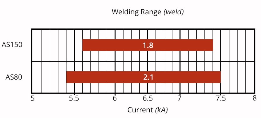
Figure 7: Influence of Aluminum-Silicon coating weight on welding range.O-16
Liquid Metal Embrittlement and Resistance Spot Welding
Cold-formable, coated, Advanced High Strength Steels are widely used in automotive applications. One welding issue these materials encounter is increased hardness in the weld area, that may result in brittle fracture of the weld. Another issue is their sensitivity to Liquid Metal Embrittlement (LME) cracking.
Both issues are discussed in detail in the Joining section of the WorldAutoSteel AHSS Guidelines website and the WorldAutoSteel Phase 2 Report on LME.
Resistance Spot Welding Using Current Pulsation
The most effective solution for these issues is using current pulsation during the welding cycle, schematically described in Figure 8.

Figure 8: Nugget growth differences in Single Pulse vs. Multi-Pulse Welding
Pulsation of the current allows much better control of the heat generation and weld nugget development. Pulsation variables include the number of pulses (typically 2 to 4), current, time for each pulse, and the cool time between the pulses.
Pulsation during Resistance Spot Welding is beneficial for press hardening steels, coated cold stamped steels of all grades, and multi-material stack-ups. Information about multi-sheet, multi-material stack-ups can be – as described in our articles on 3T/4T and 5T Stack-Ups
For more information about PHS grades and processing, see our Press Hardened Steel Primer.
Thanks are given to Eren Billur, Ph.D., Billur MetalForm for his contributions to the Equipment section, as well as many of the webpages relating to Press Hardening Steels at www.AHSSinsights.org.


