Simulation Inputs

Simulation Inputs


Predicting metal flow and failure is the essence of sheet metal forming simulation.  Characterizing the stress-strain response to metal flow requires a detailed understanding of when the sheet metal first starts to permanently deform (known as the yield criteria), how the metal strengthens with deformation (the hardening law), and the failure criteria (for example, the forming limit curve). Complicating matters is that each of these responses changes as three-dimensional metal flow occurs, and are functions of temperature and forming speed. 

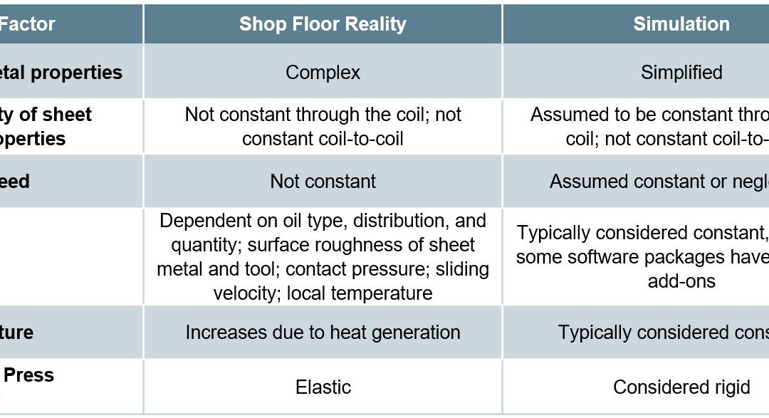
The ability to simulate these features reliably and accurately requires mathematical constitutive laws that are appropriate for the material and forming environments encountered. Advanced models typically improve prediction accuracy, at the cost of additional numerical computational time and the cost of experimental testing to determine the material constants. Minimizing these costs requires compromises, with some of these indicated in Table I created based on Citation R-28.

Table I: Deviations from reality made to reduce simulation costs. Based on Citations B-16 and R-28.

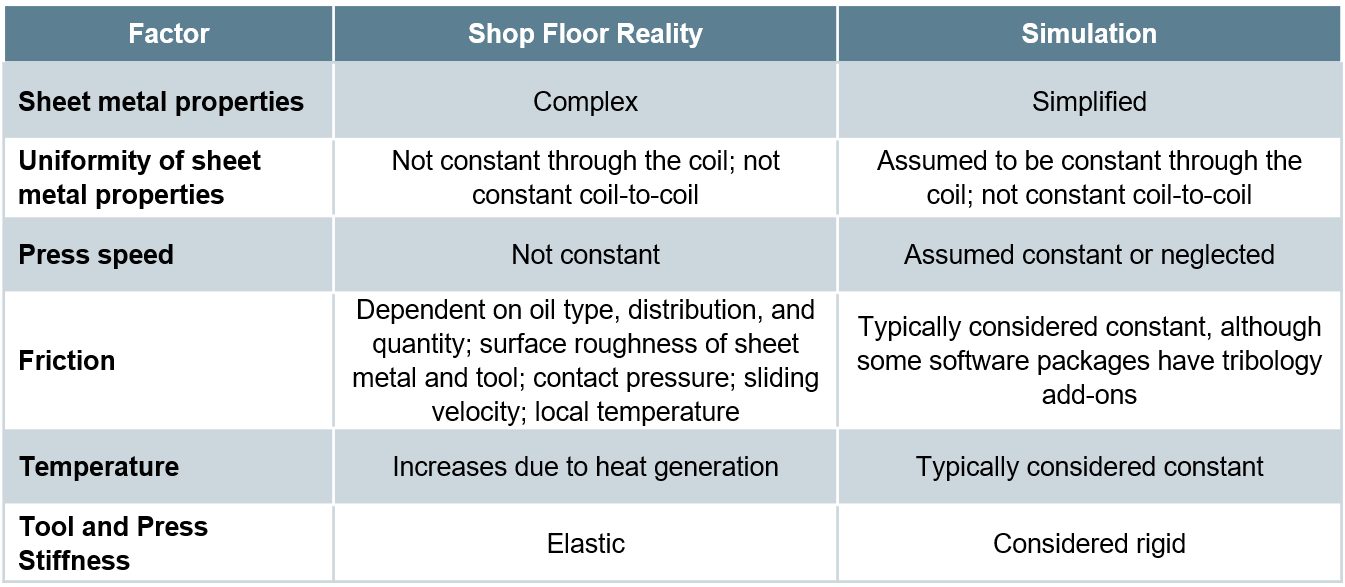
Table I: Deviations from reality made to reduce simulation costs. Based on Citation R-28.


Yield Criteria

The yield criteria (also known as the yield surface or yield loci) defines the conditions representing the transition from elastic to plastic deformation.  Assuming uniform metal properties in all directions allows for the use of isotropic yield functions like von Mises or Tresca. A more realistic approach considers anisotropic metal flow behavior, requiring the use of more complex yield functions like those associated with Hill, Barlat, Banabic, or Vegter.   

No one yield function is best suited to characterize all metals. Some yield functions have many required inputs.  For example, “Barlat 2004-18p” has 18 separate parameters leading to improved modeling accuracy – but only when inserting the correct values. Using generic textbook values is easier, but negates the value of the chosen model.  However, determining these variables typically is costly and time-consuming, and requires the use of specialized test equipment.


Hardening Curve

Metals get stronger as they deform, which leads to the term work hardening. The flow stress at any given amount of plastic strain combines the yield strength and the strengthening from work hardening.  In its simplest form, the stress-strain curve from a uniaxial tensile test shows the work hardening of the chosen sheet metal. This approach ignores many of the realities occurring during forming of engineered parts, including bi-directional deformation.

Among the simpler descriptions of flow stress are those from Hollomon, Swift, and Ludvik.  More complex hardening laws are associated with Voce and Hockett-Sherby. 

The strain path followed by the sheet metal influences the hardening. Approaches taken in the Yoshida-Uemori (YU) and the Homogeneous Anisotropic Hardening (HAH) models extend these hardening laws to account for Bauschinger Effect deformations (the bending-unbending associated with travel over beads, radii, and draw walls).

As with the yield criteria, accuracy improves when accounting for three-dimensional metal flow, temperature, and forming speed, and using experimentally determined input parameters for the metal in question rather than generic textbook values. 


Failure Conditions

Defining the failure conditions is the other significant challenge in metal forming simulation. Conventional Forming Limit Curves describe necking failure under certain forming modes, and are easier to understand and apply than alternatives. Complexity and accuracy increase when accounting for non-linear strain paths using stress-based Forming Limit Curves.  Necking failure is not the only type of failure mode encountered. Conventional FLCs cannot predict fracture on tight radii and cut edges, nor can they account for dimensional issues like springback.  For these, failure criteria definitions which are more mathematically complex are appropriate.


Constitutive Laws

Simple material models reduce the effort of testing, but may not be sufficiently accurate or do not apply to the spectrum of grades available today.

The yield surface constructed with Hill’48H-74 requires only data from three tensile tests. Models like Barlat-1989B-89, Barlet-2003B-90, Barlat-2005B-91,  BBC2005B-92, VegterV-26, and Vegter liteV-27 all require data from more detailed advanced tests, but simulation results incorporating these yield surfaces more closely match experimental results.

Use caution with the assumptions that go into the Material Card.  For example, the card may show the r-value in the rolling, diagonal, and transverse (0°, 45°, and 90°) orientations all the same (not realistic), or worse yet, all equal to 1. For high strength and advanced high strength steels, it is likely that at least one of the orientations will have an r-value below 1. In these cases assuming an r-value of 1 will lead to an underestimation of the thinning.  Furthermore, use of the Hill 1948 yield criterion is not recommended since the model assumptions do not apply to r-values of less than 1.

The Keeler equation for FLC0 K-71 requires only the n-value and thickness, but is based on a correlation established from grades and testing available no later than the early 1990s.

Predictive models for the yield surfaceA-96 and FLCsA-97 in cold stamping conditions were created to simplify the testing requirements while maintaining the accuracy and usefulness of these advanced models. These predictive equations have been validated against physical testing for mild steels, conventional high strength steels, advanced high strength steels, aluminum alloys, and stainless steel grades. 

Similarly, for hot stamping, predictive models based on conventional tensile testing have been developed and verified.A-94, D-48, A-98  Challenges here include that elongation and r-value both vary with temperature and testing speed.

On the Forming Limit Curve shown in Figure 1a, the uniaxial strain path, plane strain, biaxial, and balanced biaxial points are predicted from total elongation (A80) and r-value determined from tensile testing in the 0, 45 and 90° orientations with respect to rolling direction.A-94 Compared with the Keeler model, the Abspoel & Scholting model is better at predicting the FLC of DP800, noting the upper limiting strains found in the experiment match the FLC, as well as a more accurate representation of the slope on the LH side.  Both models appear sufficient for the conventional grade DC04 (similar to CR3).

Figure 1. a) FLC prediction locations. b) FLC comparison on drawing steel DC04 (CR3); c) FLC comparison on DP800.A-94

Figure 1. a) FLC prediction locations. b) FLC comparison on drawing steel DC04 (CR3); c) FLC comparison on DP800.A-94


Yield surface correlations use Tensile strength (Rm), uniform elongation (Ag) and r-value test data as inputs to predict the equi-biaxial, plane strain and shear points in three directions. Figure 2 compares biaxial yield strength predictions between Hill’48 and Vegter 2017, showing the improved correlation in the model developed almost 70 years later.

Figure 2. Comparison of measured biaxial yield strength with prediction from Hill’48 (red) and Vegter 2017 (yellow).A-94

Figure 2. Comparison of measured biaxial yield strength with prediction from Hill’48 (red) and Vegter 2017 (yellow).A-94


Figure 3 presents a comparison of the measured yield surfaces of DX54D+Z (galvanized CR3) and DP1000 with those predicted by Hill’48 and Vegter 2017, highlighting the improved accuracy found in Vegter 2017.

Figure 3. Comparison of measured yield surface with predictions from Hill’48 and Vegter 2017. a) DX54D+Z (galvanized CR3); b) DP1000.A-94

Figure 3. Comparison of measured yield surface with predictions from Hill’48 and Vegter 2017. a) DX54D+Z (galvanized CR3); b) DP1000.A-94


Material properties like elongation, r-value, the hardening curve, and forming limits are all likely both strain-rate and temperature dependent, meaning that a rate-dependent and temperature-dependent yield surface and forming limit curve are needed for more accurate representations of cold- and hot-stamping.

The initial implementation of the Vegter yield surface in forming simulation software packages showed satisfactory correlation with conventional stamping applications, but was sub-optimal in operations where stresses are found in the thickness direction such as coining, wall ironing and score forming processes in packaging and battery applications. In these cases, a non-convexity close to the equi-biaxial point of the yield locus was observed, likely due to extreme anisotropy or very low r-values.

Citation A-95 discusses methods for improved accuracy. DIC measurements offer improved r-value characterization over mechanical measurement approaches. Yield locus correlations at low and high plastic strain ratios were also improved. Shell elements used in the simulation of the yield surface in plane stress ignore the strains in the through-thickness direction. For the applications where thickness stresses play a role (like wall ironing, coining, score forming in packaging, and sharp radii in closures, solid or thick shell elements are required.  The yield surface was extended to the thickness direction to allow for improved characterization in these applications having significant stresses through the thickness. This extension may be deployed in forming simulation software as “Vegter 2017.1.”


Constitutive Laws and Their Influence on Forming Simulation Accuracy

Many simulation packages allow for an easy selection of constitutive laws, typically through a drop-down menu listing all the built-in choices. This ease potentially translates into applying inappropriate selections unless the simulation analyst has a fundamental understanding of the options, the inputs, and the data generation procedures.

Some examples:

  • The “Keeler Equation” for the estimation of FLC0 has many decades of evidence in being sufficiently accurate when applied to mild steels and conventional high strength steels. The simple inputs of n-value and thickness make this approach particularly attractive.  However, there is ample evidence that using this approach with most advanced high strength steels cannot yield a satisfactory representation of the Forming Limit Curve.
  • Even in cases where it is appropriate to use the Keeler Equation, a key input is the n-value or the strain hardening exponent. This value is calculated as the slope of the (natural logarithm of the true stress):(natural logarithm of the true strain curve). The strain range over which this calculation is made influences the generated n-value, which in turn impacts the calculated value for FLC0.
  • The strain history as measured by the strain path at each location greatly influences the Forming Limit. However, this concept has not gained widespread understanding and use by simulation analysts.
  • A common method to experimentally determine flow curves combines tensile testing results through uniform elongation with higher strain data obtained from biaxial bulge testing. Figure 4 shows a flow curve obtained in this manner for a bake hardenable steel with 220 MPa minimum yield strength.  Shown in Figure 5 is a comparison of the stress-strain response from multiple hardening laws associated with this data, all generated from the same fitting strain range between yield and tensile strength.  Data diverges after uniform elongation, leading to vastly different predictions. Note that the differences between models change depending on the metal grade and the input data, so it is not possible to say that one hardening law will always be more accurate than others.
Figure 1: Flow curves for a bake hardenable steel generated by combinng tensile testing with bulge testing L-20

Figure 4: Flow curves for a bake hardenable steel generated by combining tensile testing with bulge testing.L-20


Figure 2: The chosen hardening law leads to vastly different predictions of stress-strain responses L-20

Figure 5: The chosen hardening law leads to vastly different predictions of stress-strain responses.L-20


  • Analysts often treat Poisson’s Ratio and the Elastic Modulus as constants.  It is well known that the Bauschinger Effect leads to changes in the Elastic Modulus, and therefore impacts springback.  However, there are also significant effects in both Poisson’s Ratio (Figure 6) and the Elastic Modulus (Figure 7) as a function of orientation relative to the rolling direction. Complicating matters is that this effect changes based on the selected metal grade.  
Figure 3:  Poisson’s Ratio as a Function of Orientation for Several Grades (Drawing Steel, DP 590, DP 780, DP 1180, and MS 1700) D-11

Figure 6:  Poisson’s Ratio as a Function of Orientation for Several Grades (Drawing Steel, DP 590, DP 980, DP 1180, and MS 1700) D-11


Figure 4:  Modulus of Elasticity as a Function of Orientation for Several Grades (Drawing Steel, DP 590, DP 780, DP 1180, and MS 1700) D-11

Figure 7:  Modulus of Elasticity as a Function of Orientation for Several Grades (Drawing Steel, DP 590, DP 980, DP 1180, and MS 1700) D-11


Testing to Determine Inputs for Simulation

Complete material card development requires results from many tests, each attempting to replicate one or more aspects of metal flow and failure. Certain models require data from only some of these tests, and no one model typically is best for all metals and forming conditions.  Tests described below include:

  • Tensile testing [room temperature at slow strain rates to elevated temperature with accelerated strain rates]
  • Biaxial bulge testing
  • Biaxial tensile testing
  • Shear testing
  • V-bending testing
  • Tension-compression testing with cyclic loading
  • Friction

Tensile testing is the easiest and most widely available mechanical property evaluation required to generate useful data for metal forming simulation. However, a tensile test provides a complete characterization of material flow only when the engineered part looks like a dogbone and all deformation resulted from pulling the sample in tension from the ends. That is obviously not realistic. Getting tensile test results in more than just the rolling direction helps, but generating those still involves pulling the sample in tension.  Three-dimensional metal flow occurs, and the stress-strain response of the sheet metal changes accordingly.  

The uniaxial tensile test generates a draw deformation strain state since the edges are free to contract.  A plane strain tensile test requires using a modified sample geometry with an increased width and decreased gauge length, 

Forming all steels involves a thermal component, either resulting from friction and deformation during “room temperature” forming or the intentional addition of heat such as used in press hardening. In either case, modeling the response to temperature requires data from tests occurring at the temperature of interest, at appropriate forming speeds.  Thermo-mechanical simulators like Gleeble™ generate such data.

Conventional tensile testing occurs at deformation rates of 0.001/sec. Most production stamping occurs at 10,000x that amount, or 10/sec. Crash events can be 2 orders of magnitude faster, at about 1000/sec.  The stress-strain response varies by both testing speed and grade. Therefore, accurate simulation models require data from higher-speed tensile testing. Typically, generating high speed tensile data involves drop towers or Split Hopkinson Pressure Bars.

A pure uniaxial stress state exists in a tensile test only until reaching uniform elongation and the beginning of necking.  Extrapolating uniaxial tensile data beyond uniform elongation risks introducing inaccuracies in metal flow simulations. Biaxial bulge testing generates the data for yield curve extrapolation beyond uniform elongation. This stretch-forming process deforms the sheet sample into a dome shape using hydraulic pressure, typically exerted by water-based fluids.  Citation I-12 describes a standard test procedure for biaxial bulge testing.

A Marciniak test used to create Forming Limit Curves generates in-plane biaxial strains.  Whereas FLC generation uses 100 mm diameter samples, larger samples allow for extraction of full-size tensile bars.  Although this approach generates samples containing biaxial strains, the extracted samples are tested uniaxially in the conventional manner.

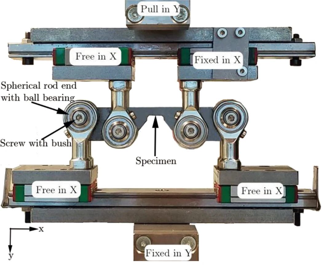
Biaxial tensile testing allows for the determination of the yield locus and the biaxial anisotropy coefficient, which describes the slope of the yield surface at the equi-biaxial stress state. This test uses cruciform-shaped test pieces with parallel slits cut into each arm. Citation I-13 describes a standard test procedure for biaxial tensile testing.  The biaxial anisotropy coefficient can also be determined using the disk compression testing as described in Citation T-21.

Shear testing characterizes the sheet metal in a shear loading condition. There is no consensus on the specimen type or testing method. However, the chosen testing set-up should avoid necking, buckling, and any influence of friction.

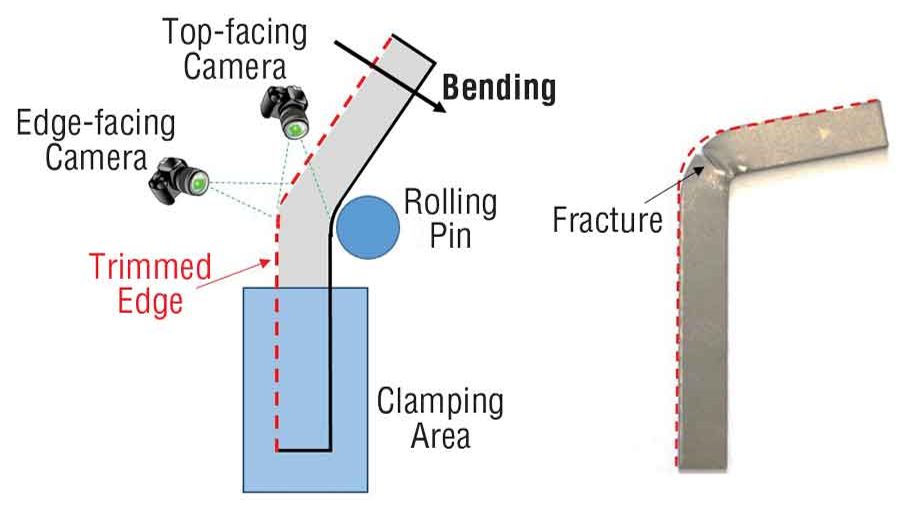
V-bending tests determine the strain to fracture under specific loading conditions. Achieving plane strain or plane stress loading requires use of a test sample with features promoting the targeted strain state. 

Tension-compression testing characterizes the Bauschinger Effect.  Multiple cycles of tension-compression loading captures cyclic hardening behavior and elastic modulus decay, both of which improve the accuracy of springback predictions. 

The Bauschinger effect leads to early re-yielding after loading reversal, and has been observed in loading-reverse loading testing.  The Yoshida-Uemori (YU) kinematic hardening model accurately captures the Bauschinger effect as well as other hardening behaviors of sheet metals during loading-reverse loading.Y-7, Y-8

Characteristics of the Bauschinger Effect (Figure 8) include a) the transient Bauschinger deformation characterized by early re-yielding and smooth elastic–plastic transition with a rapid change of the work hardening rate; b) the permanent softening characterized by a stress offset observed in a region after the transient period; and c) work-hardening stagnation appearing at a certain range of reverse deformation.Y-7

Figure 5: Characteristics of the Bauschinger Effect during cyclic loading. Y-7

Figure 8: Characteristics of the Bauschinger Effect during cyclic loading.Y-7


Citation L-78 describes an approach to calibrate the YU model on a QP1500 steel that uses a combination of physical testing and machine learning to achieve loading-reverse loading stress-strain curves over broader strain ranges.  This citation also reported that the results from tension-compression testing were not the same as those from compression-tension testing – meaning that the order of deformation influences the results.

However, no standard procedure exists for determining the kinematic hardening and Bauschinger parameters and subsequently incorporating it into metal forming simulation codes. Independent of the procedure, one of the biggest challenges with this test is preventing buckling from occurring during in-plane compressive loading. Related to this is the need to compensate for the friction caused by the anti-buckling mechanism in the stress-strain curves.

Friction is obviously a key factor in how metal flows.  However, there is no one simple value of friction that applies to all surfaces, lubricants, and tooling profiles. The coefficient of friction not only varies from point to point on each stamping but changes during the forming process. Determining the coefficient of friction experimentally is a function of the testing approach used. The method by which analysts incorporate friction into simulations influences the accuracy and applicability of the results of the generated model.

Studies are underway to reduce the costs and challenges of obtaining much of this data. It may be possible, for example, to use Digital Image Correlation (DIC) during a simple uniaxial tensile testing to quantify r-value at high strains, determine the material hardening behavior along with strain rate sensitivity, assess the degradation of Young’s Modulus during unloading, and use the detection of the onset of local neck to help account for non-linear strain path effects.S-110


Application of Advanced Testing to Failure Predictions

Global formability failures occur when the forming strains exceed the necking forming limit throughout the entire thickness of the sheet. Advanced steels are at risk of local formability failures where the forming strains exceed the fracture forming limit at any portion of the thickness of the sheet.

Fracture forming limit curves plot higher than the conventional necking forming limit curves on a graph showing major strain on the vertical axis and minor strain on the horizontal axis.  In conventional steels the gap between the fracture FLC and necking FLC is relatively large, so the part failure is almost always necking.  The forming strains are not high enough to reach the fracture FLC.

In contrast, AHSS grades are characterized by a smaller gap between the necking FLC and the fracture FLC.  Depending on the forming history, part geometry (tight radii), and blank processing (cut edge quality), forming strains may exceed the fracture FLC at an edge or bend before exceeding the necking FLC through-thickness.  In this scenario, the part will fracture without signs of localized necking.

A multi-year study funded by the American Iron and Steel Institute at the University of Waterloo Forming and Crash Lab describes a methodology used for forming and fracture characterization of advanced high strength steels, the details of which can be found in Citations B-11, W-20, B-12, B-13, R-5, N-13 and G-19.

This collection of studies, as well as work coming out of these studies, show that relatively few tests sufficiently characterize forming and fracture of AHSS grades.  These studies considered two 3rd Gen Steels, one with 980MPa tensile strength and one with 1180MPa tensile.

  • The yield surface as generated with the Barlat YLD2000-2d yield surface (Figure 9) comes from:
    • Conventional tensile testing at 0, 22.5, 45, 67.5, and 90 degrees to the rolling direction, determining the yield strength and the r-value;
    • Disc compression tests according to the procedure in Citation T-21 to determine the biaxial R-value, rb.
Figure 5: Tensile testing and disc compression testing generate the Barlat YLD2000-2d yield surface in two 3rd Generation AHSS Grades B-13

Figure 9: Tensile testing and disc compression testing generate the Barlat YLD2000-2d yield surface in two 3rd Generation AHSS Grades B-13


  • Creating the hardening curve uses a procedure detailed in Citations R-5 and N-13, and involves only conventional tensile and shear testing using the procedure included in Citation P-15.
Figure 6: Test geometries for hardening curve generation. Left image: Tensile; Right image: Shear.  N-13

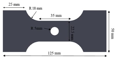
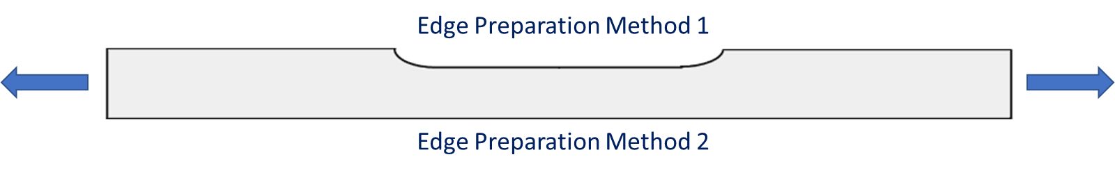
Figure 10: Test geometries for hardening curve generation. Left image: Tensile; Right image: Shear.N-13


  • Characterizing formability involved generating a Forming Limit Curve using Marciniak data or process-corrected Nakazima data. (See our article on non-linear strain paths) and Citation N-13 for explanation of process corrections].  Either approach resulted in acceptable characterizations.
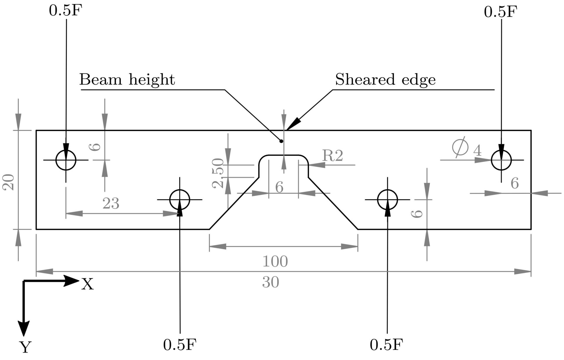
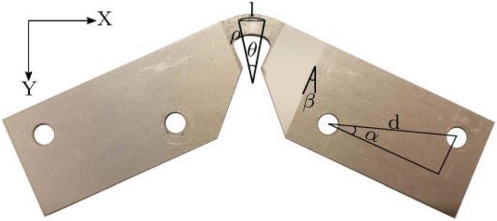
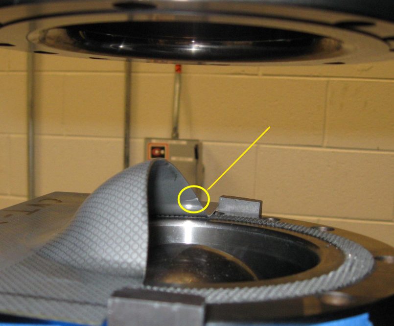
  • Fracture characterization uses four plane stress tests: shear, conical hole expansion, V-bending, and a biaxial dome test.  The result from these tests calibrate the fracture locus describing the stress states at fracture.


A different approach requires only the results from conventional tensile testing and a crack growth test under simple loading to simulate post-necking strain hardening behavior and ductile fracture.  The details of this approach are beyond the scope of this webpage, but are presented in detail in Citations S-124 and T-56, in addition to verification procedures.


Simulation Set-Up Parameters

One of the most basic choices when starting a simulation run is the setting related to the mesh size. Reduced processing time is associated with large mesh sizes, but that risks not having sufficiently fine mesh resolution to capture the forming strain gradient.  A large mesh size averages the strains over a larger region, which is analogous to a tensile bar with an 80 mm gauge length having lower elongation than a 50 mm tensile bar cut from the same sheet steel.

Figure 11 compares the Forming Limit Curve (FLC) for an 1180 MPa steel determined from gauge lengths of 2, 6, and 10 mm, along with the associated theoretical predictions. As expected, the smaller gauge length is able to more effectively capture peak strains, and is therefore associated with a higher forming limit.A-90

Figure 7: Comparison of predicted values and experimental values of the Forming Limit Curve of an 1180 MPa steel. A-90

Figure 11: Comparison of predicted values and experimental values of the Forming Limit Curve of an 1180 MPa steel.A-90


The stress-strain curve of a 1.6 mm 980 MPa steel tested with a 50 mm gauge length (ISO III, JIS) was captured, resulting in a strain at fracture of 0.147. A model based on a 2 mm element size was created, calibrated to the same strain at fracture of 0.147.  The model was re-run with element sizes of 3 mm and 5 mm, which resulted in different stress strain curves and simulations that could not predict the fracture known to occur, Figure 12. This study also showed a technique that can be used to achieve similar performance nearly independent of mesh size, such that accuracy is not compromised when optimizing computer processing speed. A-90

Figure 8: Comparison of the tensile test result and fracture model predictions based on different element sizes. A-90

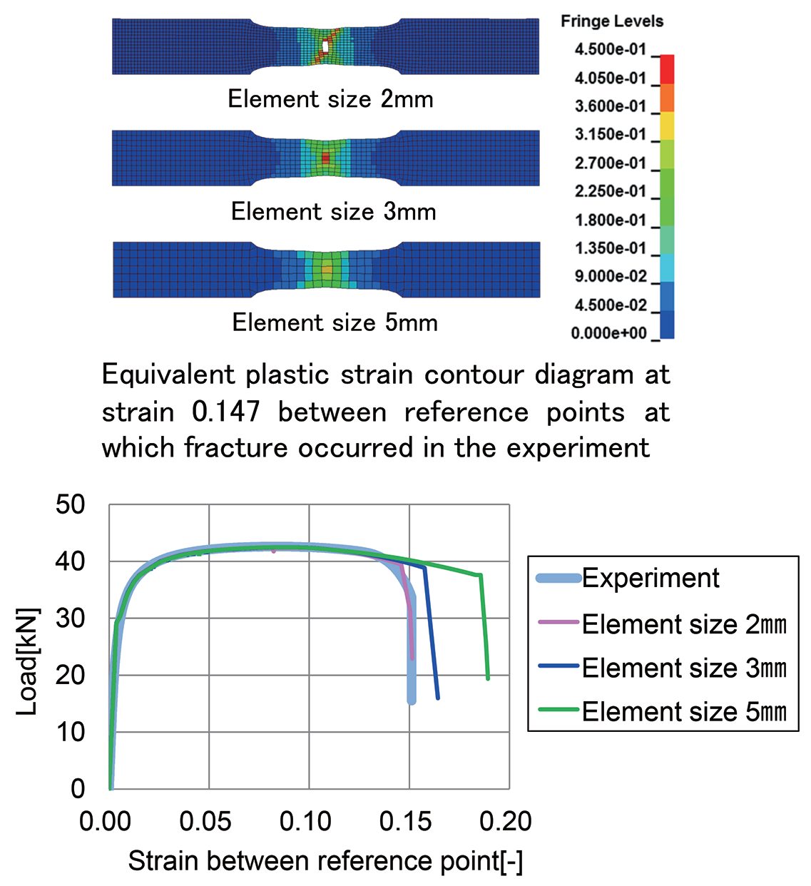
Figure 12: Comparison of the tensile test result and fracture model predictions based on different element sizes.A-90


Constitutive Models

Constitutive models for steel strengthening fall into two general categories:  power law behavior like HollomonH-71 and SwiftS-119 or saturation models like Voce and Hockett-Sherby.H-72  As shown in Figure 2 above, the chosen constitutive model significantly influences the extrapolation of experimental stress-strain curves to larger strain values. Model combinations such as Swift-Voce or Swift/Hockett-Sherby, typically using one for lower strains and the other for higher strains, typically provide better fit with experimental dataK-65, but more parameters are usually beneficial, especially for advanced high strength steels where the n-value is not constant with strain.

To improve the modeling accuracy of high strength steels with variable instantaneous nvalue, hardening curves obtained with uniaxial tensile and hydraulic bulge tests were fit to a new proposed modelL-73 to verify its predictive capability and accuracy. This new model, based on the Swift power law (Equation 1), addresses the decrease in n-value at larger plastic strains by varying what has been termed as the strain hardening attenuation coefficient a, within a new parameter λh as defined in Equation 2.

Equation 1
Equation 1
Equation 2 in Sim
Equation 2

 
When a=0, Equation 1 reverts to the standard Swift equation. When a>0, it allows for Equation 1 to correct for the decrease of instantaneous n value occurring at larger plastic strains.  The results in Figure 133 show that the predictive accuracy of the new model is better than the individual Swift or Hockett-Sherby models.

Figure 7: Hardening Curve for two grades showing Uniaxial Tensile (ut) stress-strain curves, biaxial tensile extension from biaxial bulge testing (bt), Swift and Hockett-Sherby model fit, and new model fit with different a parameter. L-73

Figure 13: Hardening Curve for two grades showing Uniaxial Tensile (ut) stress-strain curves, biaxial tensile extension from biaxial bulge testing (bt), Swift and Hockett-Sherby model fit, and new model fit with different a parameter.L-73


Experimental hardening data for a QP grade, referred to as QP1180-EL, was obtained from uniaxial tensile testing combined with bulge testing and in-plane torsion testing for strains beyond uniform elongation.  These are shown as squares and black or red circles in Figure 14, along with projections from the Swift and Hockett-Sherby models.  The Modified Power Law (MPL) achieves the best fit to the tested results.Z-18

Figure 8: Experimental results compared with the Swift power law hardening model, Hockett-Sherby saturation hardening model, and a newly developed Modified Power Law.Z-18

Figure 14: Experimental results compared with the Swift power law hardening model, Hockett-Sherby saturation hardening model, and a newly developed Modified Power Law.Z-18


Improved vehicle crashworthiness predictions occur when the forming history of the critical structural parts, including the effects of bake hardening, work hardening, and thickness reduction, are incorporated into vehicle virtual development models. Historically, simulations did not contemplate the initial damage caused by plastic deformation.  Accumulated damage can be captured within a GISSMO (Generalized Incremental Stress State Dependent Model) damage model, albeit with certain assumptions.N-30, N-31

Five different loading cases capturing the stress state of shear, uniaxial tension, stretching, plane strain and equi-biaxial stretching can be used to calibrate parameters of the Modified Mohr-Coulomb (MMC) B-83 fracture model. Schematics of these five individual tests are shown in Figure 15.H-73   The calibrated MMC model and loading path results from these tests are shown in Figure 16.  The MMC model was subsequently used to calibrate a GISSMO damage model.

Figure 9: Tests coupons for fracture model calibration. H-73

Figure 15: Tests coupons for fracture model calibration.H-73


Figure 10. Calibrated MMC fracture model and loading path results from the tests shown in Figure 9. H-73

Figure 16. Calibrated MMC fracture model and loading path results from the tests shown in Figure 10.H-73


Quasi-static three-point quasi-static bending tests were used to validate the MPL hardening model, the MMC fracture model, and the GISSMO damage model.   An FEA model with a 2 mm mesh size was compared with one having a 5 mm mesh size for the simulation of the bending process. Figure 17 shows the predicted fracture location and test result.

Local necking was observed during the experimental bending test and 2 elements failed in when using a 2 mm mesh size, yet no failure was observed when using a 5 mm mesh. This indicates that accurate simulation results may require refined mesh sizes.

Figure 11: Experiment and simulation results of three-point bending testing of a Quenched & Partitioned 1180 MPa Steel H-73

Figure 17: Experiment and simulation results of three-point bending testing of a Quenched & Partitioned 1180 MPa Steel.H-73


A subsequent studyZ-18 confirmed that ignoring the stamping forming history in the damage model results in a lower prediction of the failure risk, especially for cold stamping high-strength steel parts under large deformation conditions.
 

Case Studies: Benefits of using Advanced Models for Springback Prediction

The output of simulations using material models that thoroughly capture the changes in metal properties occurring during forming are more likely to match reality than those simulations based on basic models.

Kinematic hardening models where the Bauschinger effect and modulus degradation are captured have been shown to be substantially more accurate in springback prediction than isotropic hardening models based on more conventional tensile testing.

Citation S-130 investigated this difference.  Different types of steels having 980 MPa or 1180 MPa minimum specified tensile strength from multiple suppliers were used to form a targeted part shape using either a draw forming process or a crash forming process. The formed panels were scanned and compared with simulation results from multiple software packages. In all cases, the simulation was capable of accurately predicting strains and the risk of necking failure. 

For springback, the type of hardening model used in the simulation appeared to correlate with prediction ability. Table 2 compares the dimensional difference between the model and a scan of the physical panel, with smaller numbers representing an improved ability to predict springback in the evaluated condition. As indicated in Table 2, models incorporating Kinematic Hardening more closely matched the actual springback seen on the scanned panels. 

Table 2: Dimensional Deviation Between Simulation and Scan as a Function of Hardening Model.S-130

Maximum Sectional Deviation
During Draw Forming (mm)
Maximum Sectional Deviation
During Crash Forming (mm)
Hardening Model
5.38 5.54 Isotropic Hardening
5.25 2.27 Yoshida
5.01 10.2 Isotropic Hardening
4.2 2.422 Hill ’48 Isotropic Hardening
4.17 3.127 Hill ’48 Isotropic Hardening
3.14 2.8 Yoshida
3.12 5.3 Yoshida
2.65 N/A Yoshida
2.3 4.2 Yoshida-Uemori
2.17 7.39 Yoshida
1.98 1.64 Yoshida-Uemori
1.797 1.952 Yoshida
1.5 2.3 Yoshida
Results compiled across multiple types of simulation software,
compared with formed parts made from different types of 980 and 1180 grades from multiple suppliers.


A modified S-shape generic panel was used to evaluate springback using a 3rd Generation Steel having a minimum specified tensile strength of 980MPa.B-98  Nearly 200 points were evaluated on the panel shown in Figure 18.  For the simulation that did not incorporate kinematic hardening, 48% of this panel were within 1 mm of the physical scanned part and 32% were within 0.5 mm.  When the simulation incorporated kinematic hardening, 94% of the points were within 1 mm and 60% were within 0.5 mm.

Figure 18: Modified S-Shape used to evaluate springback on 3rd Gen 980 MPa steel in Citation B-98.

Figure 18: Modified S-Shape used to evaluate springback on 3rd Gen 980 MPa steel in Citation B-98.


A generic B-pillar panel was used to evaluate springback using a 3rd Generation Steel having a minimum specified tensile strength of 1180MPa.K-72  

For the simulation that did not incorporate kinematic hardening, 59.9% of this panel were within 1 mm of the physical scanned part.  When the simulation incorporated kinematic hardening, 68.9% of the points were within 1 mm.  Simulation results are presented in Figure 19.

Figure 19: Springback results on a B-pillar formed from 3rd Gen 1180 MPa steel.K-72 https://ahssinsights.org/citations/k-72/

Figure 19: Springback results on a B-pillar formed from 3rd Gen 1180 MPa steel.K-72 


Back To Top


Tube Forming

Tube Forming

Manufacturing precision welded tubes typically involves continuous roll forming followed by a longitudinal weld typically created by high frequency (HF) induction welding process known as electric resistance welding (ERW) or by laser welding.

Tubular components can be a cost-effective way to reduce vehicle mass and improve safety. Closed sections are more rigid, resulting in improved structural stiffness. Automotive applications include seat structures, cross members, side impact beams, bumpers, engine subframes, suspension arms, and twist beams. All AHSS grades can be roll formed and welded into tubes with large D/t ratios (tube diameter / wall thickness); tubes having 100:1 D/t with a 1mm wall thickness are available for Dual Phase and TRIP grades.

Figure 1: Automotive Applications for Tubular Components.A-35

Figure 1: Automotive Applications for Tubular Components.A-35


As roll formed and welded tubes are used with mounting brackets and little else in some Side Intrusion Beams (Figure 2), or they can be used as a precursor to hydroforming, such as the Engine Cradle shown in Figure 3.

Figure 2: Side intrusion beams made from a welded tube with mounting brackets.S-34

Figure 2: Side intrusion beams made from a welded tube with mounting brackets.S-34


Figure 3: The stages of a Hydroformed Engine Cradle: A) Straight Tube, B) After bending; C) After pre-forming; D) Hydroformed Engine Cradle. S-35

Figure 3: The stages of a Hydroformed Engine Cradle: A) Straight Tube, B) After bending; C) After pre-forming; D) Hydroformed Engine Cradle. S-35


The processing steps of tube manufacturing affect the mechanical properties of the tube, increasing the yield strength and tensile strength, while decreasing the total elongation. Subsequent operations like flaring, flattening, expansion, reduction, die forming, bending and hydroforming must consider the tube properties rather than the properties of the incoming flat sheet.

The work hardening, which takes place during the tube manufacturing process, increases the yield strength and makes the welded AHSS tubes appropriate as a structural material. Mechanical properties of welded AHSS tubes (Figure 4) show welded AHSS tubes provide excellent engineering properties. AHSS tubes are suitable for structures and offer competitive advantage through high-energy absorption, high strength, low weight, and cost efficient manufacturing

Figure 4: Anticipated Properties of AHSS Tubes; A) Yield Strength, B) Total Elongation.R-1

Figure 4: Anticipated Properties of AHSS Tubes; A) Yield Strength, B) Total Elongation.R-1


The degree of work hardening, and consequently the formability of the tube, depends both on the steel grade and the tube diameter/thickness ratio (D/T) as shown in Figure 5. The degree of work hardening influences the reduction in formability of tubular materials compared with the as-produced sheet material. Furthermore, computerized forming-process development utilizes the actual true stress-true strain curve of steel taken from the tube, which is influenced by the steel grade, tube diameter, and forming process.

Figure 5: Examples of true stress – true strain curves for AHSS tubes made from Dual Phase Steel with 590 MPa minimum tensile strength.A-36

Figure 5: Examples of true stress – true strain curves for AHSS tubes made from Dual Phase Steel with 590 MPa minimum tensile strength.A-36


Bending AHSS tubes follows the same laws that apply to ordinary steel tubes. Splitting, buckling, and wrinkling must all be avoided. As wall thickness and bend radius decrease, the potential for wrinkling or buckling increases.

One method to evaluate the formability of a tube is the minimum bend radius. An empirically derived formulaS-36  for the minimum Centerline Radius (CLR) considers both tube diameter (D) and total elongation (A) determined in a tensile test with a proportional test specimen, and assumes tube formation via rotary draw bending:

The formula shows that a bending radius equal to the tube diameter (1xD) requires a steel with 50% elongation. Successfully bending low elongation material needs a greater bend radius. Consider, for example, a dual phase steel grade where the elongation of a sample measured off the tube is 12.5%. Here, the minimum bend radius is 4 times the tube diameter. The tube bending method, the use and type of mandrels, and choice of lubrication may all affect the CLR.

The engineering strain on the outer surface can be estimated as the tube diameter (D) divided by twice the Centerline Radius (CLR):

For example, if you are bending a 40 mm diameter tube around a centerline radius of 100mm, the engineering strain on the outer surface is approximately 40/[2*100] = 20%. As a rough estimate, successful bending requires the tube to have a minimum elongation value from a tensile test in excess of this amount. Otherwise, a larger radius or modifications to the forming process is needed.

Springback is related to the elastic behavior of the tube. Yield strength variation between production batches can lead to variation in the amount of springback. A rule of thumb is that a variation of ± 10 MPa in yield strength causes a variation of approximately ± 0.1° in the bending radius. In addition, a high frequency weld which is harder and stronger than the base material causes a maximum of approximately ± 0.1° variation in bending radius.S-36

The bending behavior of tube depends on both the tubular material and the bending technique. The weld seam is also an area of non-uniformity in the tubular cross section, and therefore influences the forming behavior of welded tubes. The recommended procedure is to locate the weld area in a neutral position during the bending operation.

Figures 6 and 7 provide examples of the forming of AHSS tubes. The discussion on Tailored Products describes tailored tubes, which may be further hydroformed.

Figure 6: Dual phase steel bent to 45 degrees with centerline bending radius of 1.5xD using booster bending. Steel properties in the tube: 610 MPa yield strength, 680 MPa tensile strength, 27% total elongation. R-1

Figure 6: DP steel bent to 45 degrees with centerline bending radius of 1.5xD using booster bending. Steel properties in the tube: 610 MPa yield strength, 680 MPa tensile strength, 27% total elongation. R-1


Figure 7: Hydroformed Engine Cradle made from a dual phase steel welded tube by draw bending with centerline bending radius of 1.6xD and a bending angle greater than 90 degrees. Steel properties in the tube: 540 MPa yield strength, 710 MPa tensile strength, 34% total elongation. R-1

Figure 7: Hydroformed Engine Cradle made from a dual phase steel welded tube by draw bending with centerline bending radius of 1.6xD and a bending angle greater than 90 degrees. Steel properties in the tube: 540 MPa yield strength, 710 MPa tensile strength, 34% total elongation. R-1


Key Points

  • Due to the cold working generated during tube forming, the formability of the tube is reduced compared to the as-received sheet.
  • The work hardening during tube forming increases the YS and TS, thereby allowing the tube to be a structural member.
  • Successful bending requires aligning the targeted radii with the available elongation of the selected steel grade.
  • The weld seam should be located at the neutral axis of the tube, whenever possible during the bending operation.
Tube Forming

Bend Testing

Tensile testing cannot be used to determine bendability, since these are different failure modes. Failure in bending is like other modes limited by local formability in that only the outermost surface must exceed the failure criteria.

ASTM E290A-26, ISO 7438I-8, and JIS Z2248J-5 are some of the general standards which describe the requirements for the bend testing of metals. In a Three-Point Bend Test, a supported sample is loaded at the center point and bent to a predetermined angle or until the test sample fractures. Failure is determined by the size and frequency of cracks and imperfections on the outer surface allowed by the material specification or the end user.

Variables in this test include the distance between the supports, the bending radius of the indenter (sometimes called a pusher or former), the loading angle which stops the test, whether the loading angle is determined while under load or after springback, and the crack size and frequency resulting in failure.

For automotive applications, the VDA238-100V-4 test specification is increasingly used. Here, sample dimension, punch tip radius, roller spacing, and roller radius are all constrained to limit variability in results. Figure 1 shows a schematic of the test.

Figure 1: Schematic of Bend Testing to VDA238-100, with Bending Angle Definition.

Figure 1: Schematic of Bend Testing to VDA238-100, with Bending Angle Definition.


This video, courtesy of Universal Grip Company,U-5 describes the support rollers in the VDA238-100 test.


Calculation of the bending angle is not always straightforward. Bending formulas such as that shown within VDA238-100 assume perfect contact between the sheet metal and the punch radius. However, experimental evidence exists showing this contact does not always occur, especially in AHSS grades.

Figure 2 presents one example testing DP600 where the punch radius is larger than the radius on the bent sheet, leading to a physical separation between the punch and sheet.L-12

This physical separation also has implications for standardized bendability characterizations. A common measure of bendability is the punch radius to sheet thickness ratio, rPUNCH/t. In higher strength grades where this punch-sheet-liftoff is likely to occur, this may lead to an overestimation of how safe a design is when the punch radius may be measurably larger (less severe) than the tighter, more extreme radius actually experienced on the sheet.

Figure 2: DP600 After Testing to VDA238-100. Note punch radius is larger than radius in bent sheet resulting in separation.L-12

Figure 2: DP600 After Testing to VDA238-100. Note punch radius is larger than radius in bent sheet resulting in separation.L-12


Furthermore, bending tests do not always result in a round bent sheet shape and constant thickness around the punch tip, especially when testing 980MPa tensile strength steel grades and higher which have low strain hardening capability. Figure 3 shows pronounced flattening and thinning of the sheet below the punch tip after bending, occurring primarily on the side opposite the punch stretched in tension. Efforts to replicate this phenomenon in simulation have failed, since the underlying mechanism is not yet fully understood.

Figure 3: Flattening and Thinning Behavior after Bending.L-12

Figure 3: Flattening and Thinning Behavior after Bending.L-12


Results from bend testing are typically reported as the smallest R/T (the ratio between the die radius and the sheet thickness) that results in a crack-free bend. Many steel companies report minimum bend test limits for various grades and certain automakers include minimum bend test requirements in their specifications as well. Different steel companies and automakers may have different bend test methods and/or requirements, so it is important to understand those requirements and procedures to better match the material characteristics with the customer’s design and process expectations. The test methods could involve a bend of 60°, 90°, 180° as well as various radii, die materials, speeds, etc.

Figure 4 shows etched cross sections of different grades bend to either 0T (fold flat) or 0.5T radii for reference purposes.

Figure 4: Etched cross sections of various grades. Top row, left: 0T bend of DP350/600; Top row, right, 0T bend of HSLA450/550; Bottom left: 0.5T bend of TRIP 350/600; Bottom center: 0T bend of TRIP 350/600; Bottom right: 0.5T bend of DP 450/800.K-1

Figure 4: Etched cross sections of various grades.  Top row, left: 0T bend of DP350/600;  Top row, right: 0T bend of HSLA450/550;  Bottom left: 0.5T bend of TRIP 350/600;  Bottom center: 0T bend of TRIP 350/600;  Bottom right: 0.5T bend of DP 450/800.K-1

Edge Stretching Tests

Edge Stretching Tests

topofpage


The ISO 16630 Hole Expansion Test and the VDA238-100 bend test are among the few standardized tests to characterize local formability, the term which describes when part and process design, in addition to sheet metal properties like strength and elongation, influence the amount of deformation the metal can undergo prior to failure.

As schematically shown in Figure 1, the stress state at the edge of the hole expansion test specimen is influenced by friction, contact forces, and out-of-plane deformation, and therefore the hole expansion ratio as determined by ISO 16630 is not solely a material characteristic.

Figure 1: Parameters influencing stress state at edge of hole expansion test specimen.K-68

Figure 1: Parameters influencing stress state at edge of hole expansion test specimen.K-68


Researchers have developed alternate tests to further investigate process parameters and more clearly understand and optimize non-steel related variables. Also important is the investigation of different strain states from the ones seen in the hole expansion and bending tests. Comparisons of the stretched or bent edge performance evaluating different process parameters using the same material help to better define optimum process parameters. Repeating the testing with different AHSS grades confirms if similar trends exist across different microstructures and strengths. Standardization of these alternate tests has not yet occurred, so use caution when comparing specific values from different studies.


Hole Tension Test (In-Plane Deformation)

Microstructural damage in the shear affected zone reduces edge ductility. Damage has been evaluated with a modified tensile dogbone containing a central hole prepared by shearing or reaming, as shown in Figure 2. In contrast with a hole expansion test using a conical punch, the researchers described this as a Hole Tension test, which determines failure strain as a function of grade and edge preparation.

Figure 1: Hole Tension Test Specimen GeometryP-12

Figure 2: Hole Tension Test Specimen GeometryP-12


Edge Tension Test (In-Plane Deformation)

A two-dimensional (2-D) edge tension test, also called Half-A-Dogbone test, also evaluates edge stretchability. There are multiple versions of this type of test, but they all are based on the same concept. Like a standard tensile test, the 2-D edge tension test pulls a steel specimen in tension until failure. Unlike a standard tensile test where both sides of the tensile specimen are milled into a “dog bone”, the 2D tension test uses half of a dogbone with different preparation methods for the straight edge and the edge containing the reduced section (Figure 3). The chosen preparation method for each face is a function of the parameter being investigated (ductility, strain, burr, and shear affected zone for example).  Potential edge preparation methods include laser cutting, EDM, water jet cutting, milling, slitting or mechanical cutting at various trim clearances, shear angles, rake angles or with different die materials.

Figure 2: 2-D Edge Tension Test Sample. Note the edges are prepared differently based on the targeted property evaluated.

Figure 3: 2-D Edge Tension Test Sample. Note the edges are prepared differently based on the targeted property evaluated.


The hole expansion test is prone to scatter in the results.  Many replicates are usually tested to improve the robustness of any conclusions.  In addition, the test averages the strains over the entire circumference, and as such is lower than the peak strain immediately surrounding the location of crack initiation. 

The Sheared Edge Tensile test (SET)W-25 has many merits:  it does not require many samples, sample preparation is relatively easy, and the test itself can be performed on a regular tensile test machine.  However, the test itself can be complicated to execute, partially because it requires stopping the test immediately after a load drop of 0.5% to 4% from peak load. Full separation of the specimen after failure is to be avoided since it can cause substantial distortion of the cross section along the failure.

This test was modified to eliminate the need to monitor and control based on load drop by using non-contact optical strain measurements facilitated by DIC (digital image correlation), creating what is termed the Sheared Edge Tensile – Improved test (SETi).A-92

A benefit of the use of DIC with SETi is that local peak strains can be captured, allowing for determination of critical strain measurements that can be fed into forming simulations.

More information about SETi can be found in Citations A-92 and A-93.


Side Bending Test (In-Plane Deformation)

Instead of a dogbone or half-dogbone, some studies use a rectangular strip without a reduced section. Bending performance can be evaluated with a rectangular strip having one finished edge and one trimmed edge while preventing out-of-plane buckling, as shown in Figure 4.G-7 

Figure 3: The side-bending test expands a trimmed edge over a rolling pin until detection of the first edge crack.G-7

Figure 4: The side-bending test expands a trimmed edge over a rolling pin until detection of the first edge crack.G-7


Another type of in-plane side bending test is described in Citation K-68. The set-up shown in Figure 5 delays necking, allowing for determination of the hardening curve above uniform elongation. A key addition to the fixture is the anti-bucking mechanism. Unlike a standard hole expansion test, there is no friction and contact stress on the edge.  The strain gradient is controlled by changing the beam height of the sample (Figure 6).  An indication of the measurable dimensions after deformation is seen in Figure 7.

Figure 5: In-plane bending test fixture.K-69

Figure 5: In-plane bending test fixture.K-69


Figure 6: Sample geometry for in-plane bending test. K-69

Figure 6: Sample geometry for in-plane bending test.K-69


Figure 7: Deformed sample after in-plane bending test.K-68

Figure 7: Deformed sample after in-plane bending test.K-68


The in-plane bending test provides more details of fracture strain in a desired material orientation relative to the rolling direction compared with the axisymmetric hole expansion test. In the hole expansion test, the weakest direction determines the result due to inherent rotational symmetry in the test. With potential anisotropy in the martensite morphology found in DP steels, the ability to improve characterization in specific orientations may be useful.

The in-plane bending test was used to show a DP800 sheared edge parallel to the transverse direction has a lower fracture strain than a sheared edge parallel to the rolling direction. Furthermore, a sharper cutting tool improves edge ductility.K-68  All tests allowed for two weeks between cutting and testing; over that two week period edge fracture strain is influenced by the time between cutting and testing, but stabilizes after two weeks.A-91 

This test also was used to explore void distribution and the uniformity of plastic deformation in sheared edges.K-70   This study shows that the blanking process creates an inhomogeneous void distribution in the thickness direction. As the deformation increases during the subsequent in-plane bending test, the micro-cracks initiate at the burr region and grow towards the rollover region. Once they entirely pass the thickness of the material, they grow further, away from the edge.

No voids are present in the relatively smoother rollover and burnish regions of the sheared edge, whereas the rougher fracture region and burr contain many voids.  The majority of voids are a result of martensite cracking and separation of ferrite–martensite interfaces. 

Overall, the initial void volume fraction inside the severely hardened layer of the as-cut edge plays a more critical role than roughness in edge ductility.  Removing the volume from edge with high void density (in this case, 40 microns) is enough to significantly increase the edge ductility. It is not necessary to remove the complete shear-affected zone, which for this study is on the order of 500 microns.


Half-Specimen Dome Test (Out-of-Plane Deformation)

Deformation in these three tests occur in the plane of the sheet.  Typical hole expansion tests, like production stampings, deform the sheet metal perpendicular to the plane of the sheet. However, hole expansion testing does not always give consistent test results. The half-specimen dome test (HSDT) also attempts to replicate this 3-dimensional forming mode (Figure 8), and appears to be more repeatable likely due to creating a straight cut rather than round hole.

In the HSDT, a rectangular blank is prepared with one edge having the preparation method of interest, like sheared with a certain clearance or laser cut or water-jet cut.  The sample is then clamped with the edge to be evaluated over a hemispherical punch.  The punch then strains the clamped sample creating a dome shape, with the test stopping with the first crack appears at the edge.  Edge stretchability is quantified by measuring dome height or edge thinning or other characteristics.

Figure 4: Half-Specimen Dome Test sample. Arrow points to edge crack.S-12

Figure 8: Half-Specimen Dome Test sample. Arrow points to edge crack.S-12


Edge Flange Test (Out-of-Plane Deformation)

Flanging limits depend on the part contour, edge quality, and material properties. Non-optimal flange lengths – either too long or too short – will lead to fracture. Different tools can assess the influence of flange length, including the one shown in Figure 9 from Citation U-3.

Figure 5: Tool design to investigate flange length before fracture. Flange height: 40mm in left image, 20mm in right image.U-3

Figure 9: Tool design to investigate flange length before fracture. Flange height: 40mm in left image, 20mm in right image.U-3


Physical tests using this tool show that optimizing sample orientation relative to the rolling direction leads to longer flange lengths before splitting.U-3 Figure 10 highlights the results from testing DP800.

Figure 6: Flange height limits as a function of orientation in DP800.U-3

Figure 10: Flange height limits as a function of orientation in DP800.U-3


Effect of Time on Edge Ductility

The time passed between cutting and deforming has a large influence on the test results.

Edge ductility test results are impacted by the amount of elapsed time between cutting and deforming.  Citation A-91 documented this effect on two coils each of galvanized or bare dual phase steels having different chemistry that were evaluated with Hole Expansion Capacity (HEC), Sheared Edge Tensile – Improved (SETi), and BMW’s Kantenriss Empfindlichkeitstest (translated to edge crack sensitivity test, abbreviated as KRE) tests.

The difference between testing a few hours versus a few days after cutting can be a reduction of up to 10 HEC%, or a true strain of 0.1.  Property values appear to be stable when tested within 4 hours after cutting or after 24 hours after cutting, at the high and low values, respectively. It was also found that this effect pertains only to zinc coated materials – no edge ductility reduction over time was found in bare steels.

A practical implication of this time effect is that a galvanized part formed in a coil-fed press line should have fewer problems with edge ductility than if blanks were prepared offline in advance, all other things being equal.

At least one automotive OEM recognizes this and puts timing restrictions on the hole expansion evaluation test procedure, stating that there must be a delay of “24 h ± 1 h at room temperature” after punching but before the hole expansion test begins to avoid the aging effect.

Making a second cut to remove the work hardened zone produced during the first cut, called shaving or pre-piercing, can improve the edge ductility.  See the bottom of our page on shearing for more information.  This practice may have the additional benefit of reducing or eliminating the time delay sensitivity associated with stretching of galvanized cut edges.

Although Citation A-91 evaluated only coated and uncoated DP steels, similar conclusions were drawn in another study covering dual phase (DP), complex phase (CP), and high strength low alloy (HSLA) grades,S-126  and another study covering DP steels of different strength levels.W-46

However, another studyC-44 observed a decrease in hole expansion capacity for galvanized complex phase steel, uncoated martensitic steel, and one galvanized dual phase grade. Yet the effect was absent in galvanized bake hardening (BH), uncoated transformation induced plasticity aided bainitic-ferritic (TBF), and another uncoated dual phase grade. A related studyC-45 concluded that the advanced high strength grades with good edge ductility were the most susceptible to a decrease in edge stretchability with aging.


Influence of Starting Dimension

In addition to the time between edge creation and testing, the starting reference dimension of the analyzed region influences the results.   Edge strains of samples from CR440Y780T-DP were evaluated using four tests: two with a relatively large strain reference length, and two associated with smaller strain reference lengths.  It is found that the measured edge formability increases with a smaller strain reference length.S-127

This is similar to the effect seen in a comparison of A80 and A50 tensile bars, where A80 – having the longer reference length – is associated with lower elongation values than on an A50 bar of the same material.

The strain reference length in physical testing should correspond to the element size in associated forming simulation.

Figure 11: Limiting edge strains of the same material tested and evaluated differently. The red bar is from a conventional ISO 16630 test, except a dome was used to expand the hole instead of a conical punch. The lighter blue bar are the results from the same test, but a non-contact DIC method was used to measure the limiting strains instead of the change in hole diameter.S-127

Figure 11: Limiting edge strains of the same material tested and evaluated differently. The red bar is from a conventional ISO 16630 test, except a dome was used to expand the hole instead of a conical punch. The lighter blue bar are the results from the same test, but a non-contact DIC method was used to measure the limiting strains instead of the change in hole diameter.S-127


Back to the Top


Tube Forming

Improvement by Metallurgical Approaches

The Hole Expansion test (HET) quantifies the edge stretching capability of a sheet metal grade having a specific edge condition. Many variables affect hole expansion performance.  By understanding the microstructural basis for this performance, steelmakers have been able to create new grades with better edge stretch capability.

Multiphase microstructures with large hardness differences between the phases, specifically islands of the very hard martensite surrounded by a softer ferrite matrix, may crack along the ferrite-martensite interface (Figure 1). The larger the size of the initiated damage site (due to edge shearing), the smaller the critical stress required for crack propagation.M-6  The microstructure and damage are key components of the Shear Affected Zone, or SAZ.

Figure 1: Features and mechanisms of damage initiation and propagation in Dual Phase steel.M-6

Figure 1: Features and mechanisms of damage initiation and propagation in Dual Phase steel.M-6


One metallurgical approach to improve sheared edge stretchability is targeting a homogeneous microstructure.  Steel suppliers have engineered product offerings like complex phase steel, where extensive grain refinement (reducing the size of the ferrite and martensite grains) is achieved. Consequently, the size of the initial damage resulting from shearing is reduced, raising the critical stress for crack propagation to higher levels and reducing the likelihood for crack propagation. Additionally, reducing the difference in hardness between the soft ferrite phase and the hard martensite phase improves the hole expansion ratio. Changes in chemistry, hot rolling conditions and intercritical annealing temperatures are some of the methods used to achieve this. Such metallurgical trends can include a single phase of bainite or multiple phases including bainite and removal of large particles of martensite. This trend is shown in Figure 2, adapted from Citation M-11.

Figure 2: Hole Expansion as a Function of Strength and Microstructure.  Adapted from Citation M-11.

Figure 2: Hole Expansion as a Function of Strength and Microstructure.  Adapted from Citation M-11.


An example of the impact of these modifications is shown in a paper published by C. Chiriac and D. HoydickC-10, where a 1 mm DP780 galvannealed steel was modified to produce a grade with improved hole expansion to achieve greater resistance to local formability failures such as edge fracture and shear fracture. These changes were made while retaining the same base metal chemistry and the same fraction of martensite in the structure, and resulted in similar tensile strength and total elongation but with a 50% increase in hole expansion (Table I and Figure 3).  The key difference is a lower martensite hardness, and a smaller difference between the hardness of the martensite and ferrite.  The modified DP grade has more homogeneous distribution of martensite with smaller ferrite and martensite grains (Figure 4).

Table I: Comparison of a conventional DP780 steel with a similar chemistry modified to improve hole expansion.C-10

Table I: Comparison of a conventional DP780 steel with a similar chemistry modified to improve hole expansion.C-10

Figure 3: Improvement in Hole Expansion improves with grade modifications and edge quality.  DMR = drilled, milled, and reamed hole; EDL = Edge Ductility Loss index, the ratio of the hole expansion of the DMR hole to that of the punched hole.C-10

Figure 3: Improvement in Hole Expansion improves with grade modifications and edge quality.  DMR = drilled, milled, and reamed hole; EDL = Edge Ductility Loss index, the ratio of the hole expansion of the DMR hole to that of the punched hole.C-10


Figure 4:  Comparison of the microstructure of a conventional DP780 steel (left) with a similar chemistry modified to improve hole expansion (right). Overall, there is the same fraction of martensite in both grades, but the modified chemistry has finer features.C-10

Figure 4:  Comparison of the microstructure of a conventional DP780 steel (left) with a similar chemistry modified to improve hole expansion (right). Overall, there is the same fraction of martensite in both grades, but the modified chemistry has finer features.C-10


A presentation at a 2020 conferenceK-16 described a study which compared DP780 from six different global suppliers. Hole expansion tests were done on 1.4 mm to 1.5 mm mm thick samples prepared with either a sheared edge at 13% clearance, a sheared edge with 20% clearance, or a machined edge. Not surprisingly, the machined edge with minimal work hardening outperformed either of the sheared edge conditions. However, when considering only the machined edge samples, the hole expansion ratio ranged from below 30% to more than 70% (Figure 5). Presumably the only difference was the microstructural characteristics of the six DP780 products.

Figure 5: Variation in hole expansion performance from DP780 from 6 global suppliers.K-16

Figure 5: Variation in hole expansion performance from DP780 from 6 global suppliers.K-56


The microstructural differences that enhance local formability characteristics may be detrimental to global formability characteristics and vice versa.  Conventional dual phase steels, with a soft ferrite matrix surrounding hard martensite islands, excel in applications where global formability is the limiting scenario.  These steels have a low YS/TS ratio and high total elongation.  However, the interface between the ferrite and martensite is the site of failures that limit the sheared edge extension of these grades.  On the other end of the spectrum, fully martensitic grades are the highest strength steels available.  These have a high YS/TS ratio, and low total elongation.  Having only a single phase helps these grades achieve surprisingly high hole expansion values considering the strength, as seen in Figure 6.

Figure 5. Hole Expansion as a Function of Edge Quality and Microstructure. Adapted from Citation H-7.

Figure 6:  Hole Expansion as a Function of Edge Quality and Microstructure. Adapted from Citation.H-7


Knowing that a higher volume fraction of martensite is needed to increase strength, combined with the awareness that minimizing the hardness differences between microstructural phases is needed to increase hole expansion (Figure 7), allows steelmakers to fine-tune their chemistry and mill processing to target specific balances of strength, tensile elongation, and cut edge expandability as measured in a tensile test.

Figure 6:  Improved Hole Expansion by Reducing the Hardness Difference between Ferrite and Martensite.H-8

Figure 7:  Improved Hole Expansion by Reducing the Hardness Difference between Ferrite and Martensite.H-8


This expands the selection of grades from which manufacturers can choose.  Traditional material selection and identification may have been based on tensile strength to satisfy structural requirements – DP980 is a dual phase steel with 980MPa minimum tensile strength.  However, newly engineered grade options offer users an extra level of refinement depending on the functional needs of the part. Products can be specified as needing high tensile elongation, high hole expansion, or a balance of these two.  In the example shown in Figure 8, note that all 3 grades have nearly identical tensile strength.

Figure 7: Engineered Microstructures Achieve Targeted Product Characteristics. (Data from Citations N-8 and F-5)

Figure 8: Engineered Microstructures Achieve Targeted Product Characteristics. (Data from Citations N-8 and F-5)


The influence of microstructure and the hardness differences between the phases is also seen in the hole expansion values of AHSS grades at strengths below 980 MPa.  A study from 2016 shows the impact of a small amount of martensite on a ferrite-bainite microstructure.N-9  Both products compared had a microstructure of 80% ferrite. In one product, the remaining phase was only bainite, while the other had both martensite and bainite.  The presence of just 8% martensite was sufficient to decrease the hole expansion capacity by 40%. (Figure 9).

Figure 8: High Hardness Differences in Microstructural Phases Decrease Edge Ductility at All Strength Levels. Adapted from Citation N-9.

Figure 9: High Hardness Differences in Microstructural Phases Decrease Edge Ductility at All Strength Levels. Adapted from Citation N-9.


Rolling direction may also influence edge fracture sensitivity on some multiphase AHSS grades. When testing a sample, edge fractures may occur first at the hole edge along the rolling direction, which corresponds to a tensile axis in the transverse direction. If the chosen grade exhibits this behavior, locate stretch flanges perpendicular to the rolling direction when possible during die and process development to increase resistance to edge fracture. If this is not practical, identify locations where inserting scallops/notches in the stretch flange will not negatively impact the part structure, fit or die processing.

During die development and die try-out, it is important to use the production-intent AHSS grade – not just one that has the same tensile strength.  Blank orientation relative to the rolling direction in these trials must also be production-intent. Often the blank die is the last completed die, so prototype blanks may be prepared by laser, EDM, water jet or even by hand during tryout.  These cutting methods will have different sheared edge extension, as measured by the hole expansion test, compared with the production-intent shearing. These differences may be sufficiently significant to prevent replication of production conditions in tryout.