Additive Manufacturing for Sheet Metal Forming Tools

Additive Manufacturing for Sheet Metal Forming Tools


Additive Manufacturing (AM) has been associated with the future of manufacturing since its inception. While it does hold several advantages in complex geometries and low-volume production, modern AM systems have yet to make significant in-roads with direct-print parts in industries like automotive manufacturing which are characterized by large volumes of relatively large metal parts. With typical volumes of 1,000+ vehicles per line per day, the required throughput of automotive factory lines outstrips what is available in current AM systems. Further, the large volume of parts allows for rapid amortization of capital equipment such as tools, dies, and stamping presses, circumventing one of the primary advantages of AM: reduced per-piece cost. However, if the focus is shifted from direct-print parts to manufacturing the supporting infrastructure, tools and dies, the economic benefits are regained. Stamping tools for Advanced High-Strength Steels (AHSS) and Press Hardened Steels (PHS) feature complex geometries and require long lead times for development and manufacturing. Using AM to manufacture forming tools for AHSS and PHS brings the opportunity for reduced tooling lead-time, reduced tooling cost, and optimization of the tools for weight, strength, and thermal management.

In this article, based on a project conducted in partnership between Honda Development & Manufacturing of America, LLC and The Ohio State University, we will survey the use of polymer and metal AM for forming tools and discuss the benefits and challenges with respect to their use in manufacturing AHSS and PHS sheet metal components.

Figure 1: Relative cost of components made via AM and traditional manufacturing methods.

Figure 1: Relative cost of components made via AM and traditional manufacturing methods.


Polymer AM Tooling

The benefits of using polymer AM dies lie within low volume production such as vehicle prototyping and spare part manufacturing where the cost of traditional tooling results in high per-piece prices.S-74, H-38  One of the most common methods of polymer AM die fabrication is Fused Filament Fabrication (FFF), also known as Fused Deposition Modeling (FDM). In the FFF process, a thermoplastic filament is fed through a heated extruder nozzle to deposit material using a CNC stage. The third dimension of the build is achieved by depositing a new layer of material on previously deposited layers. The wide variety of applicable feedstock materials and relatively simple systems make FFF a widely used modality. FFF materials relevant to forming AHSS include polylactic acid (PLA), acrylonitrile butadiene styrene (ABS), polyether ether ketone (PEEK) and polycarbonate (PC) among many others. Various additives used in FFF polymers address issues such as temperature resistance, strength, and stiffness. The most common additives for enhancing mechanical properties are carbon and glass fiber. With notable exceptions, build volumes for commercial FFF systems is typically limited, requiring full-sized dies to be pieced together from multiple builds.

Big Area Additive Manufacturing (BAAM) has also been investigated for use in creating polymer AM forming dies.H-39  BAAM is similar to FFF in that heated thermoplastic is extruded through a nozzle and positioned layer-by-layer via a CNC system. Rather than a spool of filament, BAAM uses thermoplastic pellets heated and deposited through an extruder similar to those used in injection molding. As a result, the applicable material base in BAAM is much wider, including polymers with modifiers and fillers not available in commercial FFF systems. A second advantage of BAAM systems is the build envelop of 6 m x 2.4 m x 1.8 m (20 ft x 8 ft x 6 ft)S-75, capable of printing production-scale automotive dies in a single piece.

Figure 2: Interior build volume of a BAAM system at the Oak Ridge National Lab Manufacturing Demonstration Facility.

Figure 2: Interior build volume of a BAAM system at the Oak Ridge National Lab Manufacturing Demonstration Facility.S-75


Polymer AM: Application in Hydroforming

Hydroforming of sheet metals is the process of forming metal components using a liquid medium at high pressure to force a metal blank into a female die. There are multiple variations of the hydroforming process, in which some processes apply the liquid medium directly to a sheet metal component, and others, such as bladder hydroforming, contain the liquid medium in a rubber bladder, using increased liquid pressure to expand the bladder to act as the upper die, forming the sheet metal part.

Hydroforming has merit as a prototyping method, as the process typically requires only one die, reducing the tooling investment significantly. Although hydroforming is generally a slower manufacturing process, this is not an issue when low volumes of parts are needed, such as in prototyping. There are concerns in utilizing the hydroforming process for prototypes when a traditional stamping process will be used for high volume production. Hydroforming has a slow and steady increase in pressure put on the sheet metal part and tool, which leads to a more uniform pressure distribution during the forming operation. This uniform pressure distribution can allow part shapes to be formed that would tear or wrinkle when attempted with traditional forming methods, leading to false impression of part formability. The uniform pressure distribution also leads to a more uniform thickness distribution across the sheet metal part, along with uniform strain-hardening and a reduction in spring back in the forming process.K-31 These characteristics result in sheet metal parts that have different properties than traditionally formed parts, and may perform better in a crash or fatigue test, giving an inaccurate representation of how a stamped part would perform. Since the hydroforming process cannot keep up with most high volume automotive production demands, the use of hydroforming is limited to prototypes, however, the prototypes may not match the performance of the final production part. Though there is cost savings in the hard tooling and process for prototyping, it may not be an acceptable prototype method for crash or other critical components where part strain history is important.

Polymer AM tooling can be combined with hydroforming to further reduce prototype costs in development. Since hydroforming has a slower, more uniform pressure distribution across the tool, there are no localized high strain areas that can cause cracks and deformation in plastic printed tools. By virtue of the hydroforming process requiring less tooling and the use polymer AM for the solitary tool, a significant reduction in cost can be achieved compared to machining a traditional prototype tool set. The amount of savings per part is dependent on tool geometry. Generally, higher part complexity, and therefore higher tool surface complexity, yields higher the potential savings when manufacturing tooling via AM. The increased savings is primarily due to a reduction in the time required to program, set-up, and machine traditional tooling, where AM tools require only a few minutes of setup and toolpath creation before printing. It has also been shown that printed tools can be utilized directly from the printer, with minimal post processing, further reducing the manpower needed to produce the tools. Finally, because printed tools are lightweight, there is less labor required to set the tooling up in the hydroforming press.H-40, F-29, A-59

Figure 3: Polymer AM tooling for hydroforming application.

Figure 3: Polymer AM tooling for hydroforming application.


There are multiple examples in industry where 3D Printed plastic tooling has been used with the hydroforming process to reduced costs and lead-time. In one example from an AM system OEM shows a printed tool that formed 400 parts, without noticeable cracking or deformation of the tool. This tool reduced the tool lead-time by 80% and cost by 70% when compared to CNC Machined tool.H-40, F-29, A-59  These savings were achieved by the ‘lights-out and hands-off manufacturing’ process that AM provides, compared to the labor intensive and skilled work required for the CNC programming and machining.

It has been shown that the combination of sheet metal hydroforming, along with 3D Printed plastic tooling, can allow a significant reduction in cost and investment for prototype sheet metal production. Although the hydroforming process allows for a lower cost part than traditional sheet metal stamping, care must be taken when selecting this process, as the final part may perform differently than a stamped part during crash or fatigue testing. If the final production process requires stamping due to process speed, then hydroforming for prototypes may mislead the designers and engineers about the viability of that part in production. Adding the use of polymer AM tools can lead to a higher reduction in prototype costs, but more investigation is needed in the area of process simulation to better understand long term viability of the printed tools.


Polymer AM: Application in Traditional Forming

In contrast to hydroforming, traditional cold forming of sheet metal components involves the use of opposing matched tooling. Further variations include crash forming and draw forming, with the difference being a sheet metal binder used to restrict the free draw-in of the sheet metal to promote in-plane stretching. The benefit of using traditional forming over hydroforming is the process time. Large capacity presses enable rapid closing of die sets and forming of sheet metal without needing to wait for fluid pressurization required for hydroforming AHSS. As a result, mechanical and servo-mechanical presses are commonly utilized in production of automotive components. By creating matched die sets from AM for prototype and low volume operations, the forming processes and stress-strain states of the resulting parts closely resemble those manufactured via existing mass production methods. Polymer AM tooling has been investigated for both crash formingH-38, S-76 and draw formingH-39, J-18 using a variety of AM systems and materials.

The use of polymer feedstock makes polymer AM components significantly less expensive than those made on metal AM systems. If the tool set design is carefully considered, polymer AM tools have been shown to be less expensive than traditional hard metal tools. Tools manufactured using FFF fulfil the technical requirements for small series forming runs and are 56 – 63 % less expensive than conventional metal tools made with 42CrMo4S-76 while metal forming tools constructed via BAAM can save as much as 45% of the cost of traditionally manufactured tool steel dies.H-39 This approach requires careful consideration of the AM tool set design, including the use of a mixed material approach using traditional metal tools for less geometrically complex components like blank holders, and reserving AM for tools with more complex geometry.J-18 If AM build resolution is sufficiently fine, finish machining may not be necessary, saving additional process cost. However, print time and resolution are inversely related: builds with fine resolution will take longer to print and have a higher cost in terms of AM machine time while coarse resolution builds such as those made on BAAM systems will have shorter print times but require CNC machining to achieve the final geometry. An additional cost saving measure can be achieved by using a sparse in-fill, or eliminating in-fill entirely on the AM build and then backfilling with an inexpensive material, such as epoxy or concrete, to regain tool rigidity and strength. This approach minimizes AM machine time and material, further reducing the cost of the printed die set.H-39

The largest concern with polymer tooling is the decreased rigidity of the dies. While engineering polymers have been shown to have sufficient strength for AHSS forming, even high stiffness polymers such as carbon fiber filled ABS and glass fiber filled PC have elastic moduli two orders of magnitude less than that of steel used for traditional forming tools.H-39 The lower modulus of polymer materials compared to steels results in higher tool deformations resulting in greater springback in the stamped parts. Die deflection is further exacerbated by measures used to reduce cost and build time, namely the reduction or elimination of the AM infill. However, if the infill is reduced and substituted for a higher stiffness backfill or metal inclusions, the overall stiffness of the AM die can be increased beyond that possible with a solid polymer print while reducing cost.H-39, S-76

Another consequence of the lower polymer modulus is tool wear with repeated forming cycles. Wear is divided into two primary categories: abrasive and adhesive wear. In considering polymers tools for sheet metal forming, abrasion is principally responsible for friction and wear.L-34 Abrasive wear occurs when hard particles at the interface between two surfaces press into or move against the surfaces under pressure, causing local deformation and material loss at the surface. Various tests such as the pin-on-disk test or draw bending test are used to calibrate the friction and wear behavior of polymer-metal material pairs. Accurate calibration of friction and wear are necessary for the correct prediction of tool life, which is an important design factor and economic consideration for polymer AM tooling.

Polymer AM dies have been demonstrated on several steel grades including DC01, CR3, CR240LA, and DP590 in gauges up to 1.6 mm thick. Studies have investigated progressive tool wear, formed part accuracy, and best design practices when using AM tooling. In forming steel sheet metal, polymer AM dies and the resulting parts are shown to have significant geometric deviations when features have radii smaller than 1.5 mm, with a majority of the die deformation occurring as the first part is formed.S-76  However, features with larger radii, especially when coupled with carbon fiber or glass fiber filled polymers, have been shown to have sub-millimeter deviation after trial runs of 100 parts.H-39

Figure 4: AM GF-PC die and punch with DP590 formed part. [REFERENCE 3]

Figure 4: AM GF-PC die and punch with DP590 formed part.H-39

While FE simulations are used to assess the feasibility of any new forming process, this is especially important with polymer tools. Simulating the forming processes with conventional steel tools is easier as they are usually modeled as rigid parts. Since polymer tools are much less stiff and generally weaker than their tool steel counterparts, it is important to estimate the stress levels and deflections of these tools. AM polymer parts have anisotropic mechanical properties resulting from their layered manufacturing process, infill pattern, and presence of reinforcements. These tools often have small internal voids which can contribute to the asymmetry of mechanical properties in tension and compression. It is crucial to characterize these materials using tension, compression, and shear tests in various orientations, to get accurate simulation results.D-26, C-18  FE simulations have also been used to predict the failure of polymer AM structures as a result of accumulated internal damageT-30, P-24 which is important to understanding polymer die life from a structural perspective.

Figure 5: FEA of a polymer AM die set showing tool stresses during forming. [REFERENCE 3]

Figure 5: FEA of a polymer AM die set showing tool stresses during forming.H-39

Metal AM Tooling

Applicable metal AM technologies for metal forming tools can be broadly classified into Directed Energy Deposition (DED) and Powder-Bed Fusion (PBF) processes.A-60, K-32 In DED process, thermal energy is directly focused on a small region to melt metallic powder or wire materials.K-33, S-77 After movement of the thermal energy source, the melted material is deposited, fused into the melted substrate, and solidifies.G-34 DED includes Laser Engineered Net Shaping (LENS), Direct Metal Deposition (DMD), Laser Metal Deposition (LMD), and Shaped Metal Deposition (SMD) systems.K-32 DED systems have material deposition rates in excess of 1200 cm3/h, but typically have a higher surface roughness, requiring post-process machining.

PBF processes differ from DED processes in that the metal powder feed stock is placed in a horizontal bed and selectively consolidated via a laser or electron beam. In between each successive layer, more powder is deposited to be melted or sintered to form the next layer.B-39, N-17  PBF can manufacture complex shapes with high accuracy (± 0.02 mm).N-18, S-78 However, this process is often slower than DED with deposition rates up to 105 cm3/h, so it is mainly used for small components.N-18

Metal AM: Application in Traditional Forming

While AM enables the flexible production of tools with lead-time reduction and minimal economic impactsG-35, W-29, the production cost for the metal AM tools is significantly higher compared to polymer AM tools and, in some cases, metal tools manufactured by conventional methods. However, cost of the AM tools can be mitigated through topology optimization.A-61 With topology optimization, parts with freeform geometry can be designed that are optimized against a specific objective, for example weight, strength, or stiffness. By reducing overall tool material while maintaining strength, build time on the AM system can be reduced, thereby lowering tool cost.

Unlike polymer AM parts, metal AM parts typically require suitable post-processing operations to attain the proper shape and surface finish.M-33, T-31 The added machining processes increase both tool lead-time and cost.

Other problems may arise in metal AM tools include thermal deformation, processing defects, and reduced fracture toughness.K-32  The thermal deformation results from the scanning heat source locally melting material and allowing it to cool, such as in DED and PBD processes. As each region solidifies, it continues to cool and contract, resulting in thermal stresses that increase as the build volume increases.K-34, M-34 The deformation can be mitigated through design of the component itself and placement of support structures. Processing defects in AM builds impact bulk mechanical properties such as tensile strength and fracture toughness.L-35, V-14  These defects are heterogeneously distributed within the AM build, resulting in lower fracture toughness and providing a propagation path for cracks.S-79, J-19 Residual stresses within the metal AM tools also adversely affect the fracture toughnessC-19, though this can be overcome with post-build heat treatments.

Potential applications of metal AM forming tools are in prototype construction or small series production, e.g. holders, flanges or medium-size adapters and reinforcing plates.S-74  AM methods have also been utilized for insertion of beads or other geometries for reinforcing/increasing the stiffness of tools.L-36  Cost typically prevents metal AM tools from being used in low-volume cold forming applications where the main tool body is printed, however, high wear components and insert applications have demonstrated significant lead-time savings over traditional manufacturing methods.L-36  Metal AM may be considered in cold forming applications where lead-time is at a premium and cost concerns are secondary. However, in instances where complex internal structures are required, the increased cost of metal AM is outstripped by the benefits it can provide over conventionally manufactured tools. One such example is a metal AM tool for white goods that utilizes high performance stainless steel for the forming surface and less expensive mild steel for the underlying structure. The resulting die, Figure 6, was constructed from less material, reducing overall machining time required to create the finish die surface.P-25

Figure 6: Metal AM die under construction and after nitriding. [REFERENCE 39]

Figure 6: Metal AM die under construction and after nitriding.P-25

Metal AM: Application in Hot Stamping

Hot stamping is an established process for fabricating structural parts with advanced steel and aluminum alloys.C-20 An important advantage of hot forming is that it requires low-forming loads and enables forming parts with high strength and minimal springback. However, the high temperatures required to form the material and the precise cooling required to ensure desirable component properties necessitate advanced tooling designs.

Bulk materials used for fabricating hot stamping dies require special properties. The tool material must exhibit high tensile strength, hardness, good corrosion resistance, a low thermal expansion coefficient, and high thermal conductivity.N-19 Traditionally, casting and machining are used to manufacture hot stamping tools, however, in recent years AM has gained significant traction due to the design freedom that it offers, especially when it comes to fabricating tools with conformal cooling channels. Reducing porosity is one of the primary remaining challenges to maximizing mechanical properties and achieving good build quality in AM components. Conventionally manufactured hot tool steels demonstrate properties of at least 1300 MPa tensile strength, 50 HRC hardness, 18 J of impact toughness and 22 W/mK of thermal conductivity. Selected AM materials should demonstrate at least these properties in order to be considered a reliable alternative.

When forming PHS, the steel sheet is heated to 900 °C – 950 °C and then transferred to an internally cooled stamping die where it is simultaneously stamped and quenched. The austenite into martensite transformation occurs when the sheet is cooled to a temperature in the range of 420 °C – 280 °C. To accomplish this transformation, the dies must be actively cooled at a minimum cooling rate of 27 °C per second.E-7  Maintaining tool temperatures below 200 °C helps ensure the proper cooling of the blank, resulting in high part strength, and prolongs the lifespan of the tools.H-41 To achieve this, the design of the cooling channels is critical, as improper channel design may cause the temperature of the tool to increase during the stamping process, causing insufficient quenching and reducing properties of the final product. Moreover, if cooling is not consistent throughout the die, non-homogeneous surface temperature may result in hot spots which interfere with proper quenching, creating non-homogenous material properties in the finished part. Metal AM processes provide the opportunity to have arbitrary cooling channel networks not possible with traditional machining methods, resulting in more efficient cooling and better end-part performance.

Hot stamp tooling with conformal cooling channels has been demonstrated with both DED and PBF AM processes. With DED processes, it is possible to attain minimum channel diameters as low as 3 mm and a minimum wall thicknesses of 2 mm. Unlike drilling straight holes, as done with traditional tool manufacturing, it is possible to design and fabricate complex cooling channels inside the die that results in homogeneous temperature distribution within the tool and the stamped parts. The improved temperature distribution leads to lower cycle times in hot stamping and subsequent improvement in process efficiency, reducing overall production costs. DED has also been combined with subtractive processes to create a hybrid manufacturing process.C-21 One example includes hot stamping dies manufactured by machining and additively building inserts with conformal cooling ducts.M-35 As a result, the additively manufactured channels cooled six times faster than the conventional drilled channels. In another example, manufactured injection molds with conformal cooling ducts by combining direct metal rapid tooling and machining.A-62

PBF processes are also used to integrate conformal cooling channels into forging dies and hot stamping tools. PBFA-63 has over 50 different process parameters that can impact the quality of the final part, creating a significant challenge in understanding process physics and developing an effective build strategy.S-51 Unlike other processes, PBF can produce lattice structures and conformal cooling channels with a high level of dimensional accuracy and surface roughness .

Regardless of the AM method, development of the internal network channels can be aided by topology optimization, a tool that offers great flexibility in designing non-intuitive, novel, and complex parts with high performance at reduced material cost.G-36  In addition to optimizing for mechanical objectives, topology optimization can also be defined such that it designs products considering performance criteria across multiple domains such as thermal and mechanical. Such multi-objective topology optimization is a powerful tool in designing metal AM tooling that takes advantage of the optimized thermal and mechanical performance made possible through AM processes.


Summary

The continued maturation of AM has enabled low-cost, rapid, and highly capable tooling for AHSS and PHS forming applications. Depending on the specific application needs and volume, there are several developed AM technologies that can provide economical forming applications in both low and high volume production. Through careful material selection, tool design, and simulation, AM tooling can become competitive with traditionally machined tooling in meeting the metal forming needs of the automotive industry.


Thanks are given the team who contributed this article:

Ryan Hahnlen Ryan Hahnlen, Honda Development & Manufacturing of America, LLC, Raymond, OH
Ben Hoffman, Honda Development & Manufacturing of America, LLC, Raymond, OH
Madhura Athale, Integrated Systems Engineering Department at Ohio State University, Columbus, OH
Taejoon Park, Integrated Systems Engineering Department at Ohio State University, Columbus, OH
Farhang Pourboghrat, Integrated Systems Engineering Department at Ohio State University, Columbus, OH Farhang Pourboghrat, Integrated Systems Engineering Department at Ohio State University, Columbus, OH

Back To Top

True Fracture Strain

True Fracture Strain

topofpage


Fracture strain values derived from standard uniaxial tension tests can be used to evaluate automotive crashworthiness and forming behavior of aluminum alloys and Advanced High-Strength Steels (AHSS).Y-10, W-24, W-25, L-22, L-23, T-22, H-15, L-24  The true fracture strain (TFS) and similar concepts have emerged recently as intrinsic measures of local formability for AHSS. TFS is the true (logarithmic) strain associated with the “zero-gage-length” elongation at fracture (e0), where e0 is a conceptual engineering strain value based on an infinitesimal gage length in a tension test, where:


true-fracture-strain-equation-1      Equation 1


and Ao and Af are the cross-section area before testing and the fracture area after testing, respectively (constant volume assumed).D-13  It follows that TFS is defined as:


true-fracture-strain-equation-2      Equation 2


TFS is related to percent reduction of area at fracture (Z, %), where:

true-fracture-strain-equation-3      Equation 3


True Fracture Strain (TFS) Measurement Methods:

Fracture Area (Af)

Tensile test samples have a rectangular cross section before testing, indicated in the left image in Figure 1.  The right image shows an idealized tension test specimen fracture surface, where five thickness measurement locations are indicated: two at the edges (ta, te); one at the center (tc), and two at the quarter-width positions (tb, td). Measured approximately at mid-thickness, wf is the fracture width. The dashed outline indicates the original specimen cross-section before testing (to·wo = Ao), and a 10-sided polygon (decagon) approximates the projected fracture area (Af), where the corners of the polygon correspond width-wise to the five thickness measurement locations.

Figure 1: Schematic representation of a tension test specimen before testing (left) and after fracture (right) viewed along the tensile axis.


From the dimensions portrayed in Figure 1, four possible methods to determine Af are indicated in Table 1—three lineal methods and one areal method.H-17 Method A uses a single thickness measurement at mid-width. Alternatively, for Method A the minimum thickness (tmin) may be used in cases where tctmin. Method B uses a weighted three-thickness average A-24 —also known as the ASTM parabolic method.H-14, H-16  Method C uses a five-thickness average. For Method D, Af is the area of the polygon depicted in the left image of Figure 1.

Table 1. Fracture Area Measurement Methods.H-17

Table 1. Fracture Area Measurement Methods.H-17 


Dimensional measurements may be made quickly and conveniently with a calibrated digital microscope equipped with focal stacking capability and linked to image analysis software. Note that tf, wf and Af are respectively: the projected thickness, the projected width, and the projected area of the fracture surface. That is, to accommodate irregular and angled fracture surface features, measurements are made with respect to a virtual plane normal to the tensile axis. Alternatively, lineal measurements may be made with a conventional microscope equipped with a dial indicator or measuring stage. In this case, continual manual refocusing may be necessary to ensure true projected dimensional measurements.  

Recently the effects of fracture area measurement method and tension test specimen type on fracture strain values were evaluated H-17. It was concluded that specimen type (i.e., width-to-thickness ratio) has a far greater impact on the consequent fracture strain value in contrast to that of measurement method. It was also advised that, when reporting fracture strain values derived from tension tests, the specimen type, the material thickness, and the fracture area measurement method be clearly indicated.


True Fracture Strain (TFS) Measurement Methods:

Fracture Types

Based solely on fracture appearance, various fracture types may be observed, with examples shown in Figure 2. H-17  The fracture type changes from Type 1 to Type 2 to Type 3 as the tension test specimen width-to-thickness ratio (wo/to) increases (left to right). Type 1 fracture is perpendicular to the tensile axis across the specimen width; Type 2 fracture is an irregular transition from Type 1 fracture to Type 3 fracture; and Type 3 fracture is aligned at an angle across the specimen width (~50-60° from the tensile axis).   

Figure 2: Various fracture types observed in uniaxial tension testing, from left to right: Type 1 fracture (wo/to = 4.5—ASTM Standard Sub-size specimen); Type 2 fracture (wo/to = 12.8—ASTM Standard specimen); and Type 3 fracture (wo/to = 16.8—JIS No. 5 Standard specimen); The original width-to-thickness ratio (wo/to) is measured within the gage section of the test specimen.  H-17

Figure 2: Various fracture types observed in uniaxial tension testing, from left to right: Type 1 fracture (wo/to = 4.5—ASTM Standard Sub-size specimen); Type 2 fracture (wo/to = 12.8—ASTM Standard specimen); and Type 3 fracture (wo/to = 16.8—JIS No. 5 Standard specimen); The original width-to-thickness ratio (wo/to) is measured within the gage section of the test specimen.H-17


A similar fracture orientation dependence on specimen width was reported for Dual Phase (DP) steels more than thirty years ago by researchers at the Colorado School of Mines.S-49  A 2018 publication W-23 confirmed this behavior for other AHSS types, and illustrated that the transitional behavior—in terms of critical width-to-thickness ratio—is material dependent.

Figure 3 shows example Type 1 and Type 3 fractures in cross-section at the mid-width position (corresponding to position tc in Figure 1). Type 1 fractures typically run at an angle through thickness (~50-55° from the tensile axis). While most Type 1 fractures resemble that shown in Figure 2 (left) and that shown in Figure 3a, occasional through-thickness chevron profiles and “cup and cone” W-23 type fractures have been observed for Type 1 fractures. Nevertheless, Type 1 fractures are roughly symmetric about a plane normal to the sheet surface at the mid-width position.

Figure 3. Examples of (a) Type 1 fracture, and (b) Type 3 fracture; Polished through-thickness cross-sections at the mid-width position; Tensile axis is horizontal.

Figure 3. Examples of (A) Type 1 fracture, and (B) Type 3 fracture; Polished through-thickness cross-sections at the mid-width position; Tensile axis is horizontal.


Type 3 fractures invariably show localized necking in through-thickness cross-section as in Figure 3b. Therefore, Type 3 fractures are roughly symmetric about a plane parallel to the sheet surface at the mid-thickness position. Type 2 fractures have both Type 1 and Type 3 characteristics at different positions across the width and thus have no overall plane of symmetry. Various degrees of damage (void formation) are observed in through-thickness cross-sections of fractured specimens— for example, Figure 3. Citation H-18 contains a detailed compendium with more information on this topic.

ElsewhereW-23, L-21 it was explained that the idealized fracture thickness profile—as depicted in the right image in Figure 1—is applicable only to smaller width-to-thickness ratios (thicker, hot-rolled materials or narrower gage sections). For thinner, cold-rolled materials, or for wider gage sections, there is often no clear fracture thickness minimum at the mid-width position. In fact, in some cases a fracture thickness maximum at mid-width has been observed. Furthermore, occasional mid-thickness delamination renders the volume-constancy assumption in question, with associated implications in Equation 1


True Fracture Strain (TFS):

Formability Classification and Rating System

In 2016 the foundation for a formability classification and rating system was introduced for AHSSH-14, where formability performance expectations are distinguished by the relationships between true fracture strain (TFS) and true uniform strain in a tension test. Such performance mapping concepts continue to be explored and modified by steelmakersH-16, W-23, L-21, D-12, W-22, V-5, R-6, S-48 by automakersH-18, H-19 and by international industry consortiums.G-20 Traditionally AHSS performance has been represented by the product of ultimate tensile strength and total elongation (UTS x TE) and relative position on the so-called “banana diagram” or Global Formability Diagram. While this conventional methodology discriminates behavioral extremes, much is lost regarding the nuances of local formability.

Intrinsic Formability Parameters

Widely considered an intrinsic measure of global formability, the true uniform strain (εu) is the logarithmic strain associated with uniform elongation (UE, %) in a uniaxial tension test, where:


true-fracture-strain-equation-4     Equation 4


Example TFS and εu values are shown for a series of 980-class AHSS (980 MPa minimum tensile strength) in Figure 4H-14. In this analysis, TFS values ranged from less than 0.5 [DP 980 (LSi)] to more than 1.0 (CP 980), and εu values ranged from 0.05 (CP 980) to 0.15 (GEN3 980). The Third Generation AHSS materials (GEN3-type) have the largest εu values, and the Multi-Phase/Complex-Phase steels (MP/CP-type) have the largest TFS values. As a group the Dual Phase steels (DP-type) have intermediate εu values and a wide range of TFS values. As illustrated in Figure 4, TFS is far greater than εu. A similar disparity between fracture strain and uniform strain was shown in Citation D-14, and no consistent relationship between the two parameters was determined.

Figure 4: True uniform strain (εu) and true fracture strain (TFS) values for a series of 980-class advanced high-strength steels; Error bars show the range among three test specimens for each material..H-14

Figure 4: True uniform strain (εu) and true fracture strain (TFS) values for a series of 980-class AHSS; Error bars show the range among three test specimens for each material.H-14


The local/global strain ratio (L/GSR) and the formability index are key parameters to guide application-specific material selection and to help set targets for future AHSS grade developments.H-14H-16 The L/GSR reflects the relative preponderance of local formability to global formability and is defined as:

true-fracture-strain-equation-5     Equation 5


The L/GSR is useful in understanding relative intrinsic formability “character”. Materials with higher relative TFS values are naturally expected to perform better under flanging, edge stretching and tight-radius bending conditions [e.g., MP 980 (LCE) and CP 980 in Figure 4], while materials with higher relative uniform strain values (i.e., higher terminal n values) are better suited for stretch forming and are able to distribute strain more uniformly (e.g., GEN3 980 and GEN3 980-HY in Figure 4).

Furthermore, the formability index (F.I. in the formula) is defined as:

true-fracture-strain-equation-6     Equation 6


This index represents an intermediate strain value between εu and TFS and provides a convenient measure of the overall formability expectation, where both local formability and global formability are considered.  As an example, Figure 5 shows an exponential relationship between F.I., and the limiting bend ratio (r/t) determined from 90° V-bend testing for the same series of 980-class AHSS represented in Figure 4.H-14  It was reasoned that in the early stages of deformation, global formability (εu) dictates the strain distribution around the punch nose, while fracture resistance is governed by local formability (TFS) in the latter stages of deformation.

Figure 5. Correlation between the limiting bend ratio (f) and the formability index (F.I.) for a series of 980-class advanced high-strength steels. A higher formability index corresponds to a lower (better) limiting bend ratio in 90° V-bend testing. H-14

Figure 5. Correlation between the limiting bend ratio (f) and the formability index (F.I.) for a series of 980-class AHSS. A higher formability index corresponds to a lower (better) limiting bend ratio in 90° V-bend testing.H-14


Local/Global Formability Map

Figure 6 illustrates the essential framework of the local/global formability map—known eponymously as the Hance diagram.H-14, D-12, G-20 Here, the dashed lines represent the boundaries between global character (L/GSR < 5), balanced character (5 < L/GSR < 10), and local character (L/GSR > 10). The continuous curves represent arbitrary iso-F.I. contours corresponding to the values indicated (in parentheses). The qualitative assessments (Poor through Excellent) indicated for each formability level are also arbitrary; however, these performance level monikers were chosen to reflect real-world experience. Portrayed in this way (in contrast to Figure 4, for example), the relationships between true fracture strain and true uniform strain are more discernable, and both the formability character and the formability level become apparent.

Figure 6: Essential framework of the local/global formability map concept. H-16

Figure 6: Essential framework of the local/global formability map concept.H-16


Case Study Using the Local/Global Formability MapH-15

The basic utility of the local/global formability map concept was demonstrated for an automotive seating system development program.H-15 In this case study, stamping trials were conducted with two 980-class AHSS (980 MPa minimum UTS designation):

  • 1.6mm 980DP(LSi): A classic Dual Phase (DP) ferrite/martensite steel with low silicon content (LSi), and 
  • 1.6mm 980MP(LCE)—a Multi-Phase (MP) steel with high yield strength and low carbon equivalent (LCE).

Basic formability parameters are summarized in Table 2 for the trial materials. Based solely on elongation values (UE, TE), one might have concluded that the formability of 980DP(LSi) would exceed that of 980MP(LCE).

Table 2. Formability Parameters for Two 980-Class AHSS.

Table 2. Formability Parameters for Two 980-Class AHSS.


However, the stamping trial results were counterintuitive and drastically different among the two trial materials. The 980DP(LSi) material exhibited severe edge-cracking in multiple locations, while the 980MP(LCE) material ran without issue. Both materials were free of necking-type failures as predicted by computer simulations (sufficient global formability). An example part overview is shown in Figure 7. Typical 980DP(LSi) edge cracks are shown in Figure 8 for a pierced/extruded hole (Location 1) and for a blanked/stretched perimetric edge (Location 2). Clearly, relative sheared-edge ductility may not simply be deduced from conventional tensile elongation values. 

Figure 7: Overview of a stamped automotive seating component [length ~ 480 mm (19 in.)]. H-15

Figure 7: Overview of a stamped automotive seating component [length ~ 480 mm (19 in.)].H-15

Figure 8: Close-up views of Location 1 (left) and Location 2 (right) identified in Figure 7 [material: 980DP(LSi)]; Location 1 is a pierced hole that was extruded during forming, and Location 2 is a blanked perimetric edge that was stretched during forming (underside with respect to Figure 7). H-15

Figure 8: Close-up views of Location 1 (left) and Location 2 (right) identified in Figure 7 [material: 980DP(LSi)]; Location 1 is a pierced hole that was extruded during forming, and Location 2 is a blanked perimetric edge that was stretched during forming (underside with respect to Figure 7).H-15

The local/global formability map coordinates of the 980DP(LSi) and 980MP(LCE) trial materials are shown in Figure 9. With reference to the framework described in Figure 6, 980DP(LSi) exhibits global/balanced character with an overall borderline rating of Fair/Good (F.I. = 0.20); while 980MP(LCE) has decidedly local character with an overall rating of Good (F.I. = 0.26). Furthermore, the TFS value of 980MP(LCE) is more than twice that of 980DP(LSi). 

Figure 9: Local/global formability map featuring three 980-class AHSS—980DP(LSi), a classic DP ferrite/martensite steel with low silicon content (LSi); 980MP(LCE), an MP steel with high yield strength and low carbon equivalent (LCE); and 980GEN3, a third generation AHSS. Image based on Citations H-15 and H-17.

Figure 9: Local/global formability map featuring three 980-class AHSS—980DP(LSi), a classic DP ferrite/martensite steel with low silicon content (LSi); 980MP(LCE), an MP steel with high yield strength and low carbon equivalent (LCE); and 980GEN3, a third generation AHSS. Image based on Citations H-15 and H-17.


As an independent confirmation of the local formability advantage of 980MP(LCE), the hole expansion ratio (HER, λ) is more than four times that of 980DP(LSi) (Table 2). A strong correlation between TFS and λ has been confirmed by several authors L-22 L-23  T-22  H-15 As the component featured in this case study is dominated by extremely challenging edge-stretching conditions, 980MP(LCE) is the clear wiser material selection. However, in applications with more demanding global formability requirements, other issues such as intolerable strain localization could arise, and a third generation AHSS might be the best choice. As an example, when contrasting 980GEN3 AHSS (third generation AHSS) to 980DP(LSi) in Figure 9, the intrinsic global and local formability parameters (εu and TFS), as well as the F.I, are approximately 50% greater.


True Fracture Strain (TFS): Alternatives to TFS

While the local/global formability map methodology was developed in the context of true fracture strain (TFS), there are other ways to represent intrinsic local formability (fracture resistance) with data derived from standard uniaxial tension tests. In the original conception (Hance diagram), true uniform strain (εu) and TFS are two points along a logarithmic strain continuum from zero to fracture, and the relationships between these values elegantly describe the formability character (local/global strain ratio) and the overall formability level (formability index). The “best” local formability parameter may be a matter of practicality or applicability, or simply a matter of preference. Each method has its strengths and weaknesses, and such fracture strain concepts continue to evolve. 

True Thinning Strain at Fracture  

The true fracture strain (TFS) value is an area-based measurement of fracture strain and thus reflects the tension test specimen width change as well as the thickness change, for better or for worse. Citation H-18 suggests that the true thinning strain at fracture (ε3f) is a more appropriate measure of local formability, where:


true-fracture-strain-equation-7     Equation 7


and to and tf are the original thickness (before testing) and final thickness (after fracture). By convention ε3f is a positive value and represents the absolute value of the true thickness strain at fracture (a negative value). Furthermore, the post-uniform portion of the fracture strain may be isolated by subtracting the uniform component of thinning strain, where:


true-fracture-strain-equation-8     Equation 8


and εu and r are the true axial uniform strain and the plastic strain ratio (normal anisotropy) measured during the tension test, respectively. Post-uniform fracture strain components might be more relevant to materials with high uniform elongation values such as TWIP steels H-18. In a similar way, the post-uniform portion of the area-based TFS value may be expressed as:


true-fracture-strain-equation-9     Equation 9


Another study W-23 concluded that: (1) area-based fracture strain measurements such as TFS result in less experimental scatter when compared to thickness-based fracture strain measurements such as ε3f, and (2) area-based measurements show less dependence upon the method by which fracture strains are determined. It appears that a single thickness measurement may misrepresent the fracture strain and that a multiple-thickness (average thickness) or area measurement approach may be more stable.

Critical Fracture Strain

Perhaps a lesser-known and under-exploited representation of fracture strain is the so-called critical fracture strain value (CFS)—introduced in 1999 for aluminum alloys in Citation Y-10 and re-visited in 2007 in the context of High-Strength Steel in Citation W-24. In concept CFS is the estimated true thinning strain at fracture, where:


true-fracture-strain-equation-10     Equation 10


In determining CFS, only the engineering stress-strain data from a uniaxial tension test are needed—that is, no post-fracture area or thickness measurements are required: eu is the engineering uniform strain value (% uniform elongation/100); sf is the engineering fracture stress; and su is the ultimate tensile strength or UTS. Figure 10 shows an example engineering stress-strain curve for a 980-class AHSS, where the parameters relevant to CFS are marked. In this example, CFS = -ln[(1-0.07/2)·(787/1015)] = 0.29.

Figure 10: Example engineering stress-strain curve for a 980-class AHSS. Here, eu is the engineering uniform strain, su is the ultimate tensile strength (UTS), sf is the engineering fracture stress, CFS is the critical fracture strain, and ε3f is the true thinning strain at fracture. 

Figure 10: Example engineering stress-strain curve for a 980-class AHSS. Here, eu is the engineering uniform strain, su is the ultimate tensile strength (UTS), sf is the engineering fracture stress, CFS is the critical fracture strain, and ε3f is the true thinning strain at fracture.


True Fracture Strain (TFS):

Correlation to Hole Expansion Ratio

In a recent studyL-5, tensile properties (80 mm gage length) and hole expansion ratio were measure for AHSS with minimum tensile strength designations ranging from 600 to 1200 MPa, and thickness between 1 and 2 mm. No particular correlation was found between the hole expansion ratio and conventional tensile properties such as uniform elongation, total elongation, n-value, and so on.

The most promising relationship was found between the hole expansion ratio (converted to logarithmic strain) and the true thinning strain at fracture in tension. This relationship is illustrated in Figure 11 for total thinning strain (ε3f, Equation 7) on the left, and for post-uniform thinning strain (ε*3f, Equation 8) on the right. In both cases, better correlation is shown for transverse tension tests rather than for longitudinal tension tests (linear fit through the origin).

Figure 11: Hole expansion ratio (logarithmic strain) as a function of true thinning strain at fracture.   Left graph: total thinning strain (e3f); Right graph: post-uniform thinning strain (e*3f).L-5

Figure 11: Hole expansion ratio (logarithmic strain) as a function of true thinning strain at fracture.   Left graph: total thinning strain (ε3f); Right graph: post-uniform thinning strain (ε*3f).L-5


While the above correlations are good, the inherent scatter associated with the hole expansion test, fracture strain measurements, and other local formability parameters may limit applicability in a production environment. Furthermore, various factors affect hole expansion in production environments, including hole preparation technique, edge condition, and cutting clearance.


Brandon Hance Thanks are given to Brandon Hance, Ph.D., who contributed this article.


Back to the Top


M-Value

M-Value

M-Value, Strain Rate Sensitivity

The strengthening of some metals changes with the speed at which they are tested. This strain-rate sensitivity is described by the exponent, m, in the modified power law equation:


where έ is the strain rate and m is the strain rate sensitivity.

To characterize the strain rate sensitivity, medium strain rate tests were conducted at strain rates ranging from 10-3/sec (commonly found in tensile tests) to 103/sec. For reference, 101/sec approximates the strain rate observed in a typical stamping. Both yield strength and tensile strength increase with increasing strain rate, as indicated Figures 1 and 2.

Figure 1: Influence of Strain Rate on Yield Strength

Figure 1: Influence of Strain Rate on Yield Strength.Y-1


Figure 2: Influence of Strain Rate on Tensile Strength

Figure 2: Influence of Strain Rate on Tensile Strength.Y-1


Up to a strain rate of 101/sec, both the YS and UTS only increased about 16-20 MPa per order of magnitude increase in strain rate. These increases are less than those measured for low strength steels. This means the YS and UTS values active in the sheet metal are somewhat greater than the reported quasi-static values traditionally reported. However, the change in YS and UTS from small changes in press strokes per minute are very small and are less than the changes experienced from one coil to another.

The change in n-value with increase in strain rate is shown in Figure 3. Steels with YS greater than 300 MPa have an almost constant n-value over the full strain rate range, although some variation from one strain rate to another is possible.

Figure 3: Influence of Strain Rate on n-value

Figure 3: Influence of Strain Rate on n-value.Y-1


Similar behavior was noted in another studyB-22 that included one TRIP steel and three DP steels. Here, DP1000 showed a 50% increase in yield strength when tested at 200/sec compared with conventional tensile test speeds. Strain rate has little influence on the elongation of AHSS at strain rates under 100/sec.

Relationship between strain rate and yield strength (left) and elongation (right)

Figure 4: Relationship between strain rate and yield strength (left) and elongation (right). Citation B-22, as reproduced in Citation D-44


Figure 5 shows the true stress-true strain curves for a processed Press Hardened Steel tested at different strain rates. The yield stress increases approximately five MPa for one order of magnitude increase in strain rate.

Figure 4: True stress-strain curves at different strain rates for 1mm thick Press Hardening Steel (PHS) after heat treatment and quenching.

Figure 5: True stress-strain curves at different strain rates for 1mm thick Press Hardening Steel (PHS) after heat treatment and quenching.V-1


The tensile and fracture response of different grades is a function of the strain rate and cannot be generalized from conventional tensile tests.  This has significant implications when it comes to predicting deformation behavior during the high speeds seen in automotive crash events.  See our page on high speed testing for more details.

Additive Manufacturing for Sheet Metal Forming Tools

Crash Management

In addition to enhanced formability, Advanced High-Strength Steels (AHSS) provide crash energy management benefits over their conventional High-Strength Steel (HSS) counterparts at similar strength levels.  Higher levels of work hardening and bake hardening at a given strength level contribute to this improvement in crash performance.

The energy required for plastically deforming a material (force times distance) has the same units as the area under the true stress-true strain curve.  This applies to all types of plastic deformation – from that which occurs during tensile testing, stamping, and crash.  The major difference between these is the speed at which the deformation takes place.

As an example, consider the press energy requirements of two grades by comparing the respective areas under their true stress – true strain curves.  The shape and magnitude of these curves are a function of the yield strength and work hardening behavior as characterized by the n-value when tested at conventional tensile testing speeds.    At the same yield strength, a grade with higher n-value will require greater press energy capability, as highlighted in Figure 1 which compares HSLA 350/450 and DP 350/600. For these specific tensile test results, there is approximately 30% greater area under the DP curve compared with the HSLA curve, suggesting that forming the DP grade requires 30% more energy than required to form a part using the HSLA grade.

Figure 1: True stress-strain curves for two materials with equal yield strength.T-3

Figure 1: True stress-strain curves for two materials with equal yield strength.T-3


The high degree of work hardening exhibited by DP and TRIP steels results in higher ultimate tensile strength than that exhibited by conventional HSS of similar yield strength. This provides for a larger area under the true stress-strain curve.  Similarly, when panels are formed from these grades, the work hardening during forming leads to higher in-panel strength than panels from HSS of comparable yield strength, further increasing the area under the stress-strain curve, ultimately resulting in greater absorption of crash energy.

Finally, the high work-hardening rate better distributes strain during crash deformation, providing for more stable, predictable axial crush that is crucial for maximizing energy absorption during a front or rear crash event.

Many AHSS are bake hardenable. The relatively large BH effect also increases the energy absorption capacity of these grades by further increasing the area under the stress-strain curve. The BH effect adds to the work hardening imparted by the forming operation. Conventional HSS do not exhibit a strong BH effect and therefore do not benefit from this strengthening mechanism.

Figure 2 illustrates the difference in energy absorption between DP and TRIP steels as a function of their yield strength determined at quasi-static tensile testing speeds.

Figure 2: Absorbed energy for square tube as function of quasi-static yield strength. T-2

Figure 2: Absorbed energy for square tube as function of quasi-static yield strength.T-2


Figure 3 shows calculated absorbed energy plotted against total elongation for a square tube component. The absorbed energy remains constant for the DP and TRIP steels but the increase in total elongation allows for formation into complex shapes.

Figure 3: Calculated absorbed energy for a square tube as a function of total elongation.T-2

Figure 3: Calculated absorbed energy for a square tube as a function of total elongation.T-2


For certain parts, conventional steels may have sufficient formability for stamping, yet lack the required ductility for the desired crash failure mode and will split prematurely rather than collapsing in a controlled manner. AHSS grades improve energy absorption by restoring a stable crush mode, permitting more material to absorb the crash energy.  The increased ductility of AHSS grades permit the use of higher strength steels with greater energy absorbing capacity in complex geometries that could not otherwise be formed from conventional HSS alloys.

Stable and predictable deformation during a crash event is key to optimizing the steel alloy selection. The ideal profile is a uniform folding pattern showing progressive buckling with no cracks (Figure 4).

Figure 4: Deformation after axial crushing.A-49

Figure 4: Deformation after axial crushing.A-49


Achieving crack-free folds is related to the local formability of the chosen alloy.  Insufficient bendability can lead to early failure (Figure 5).  Research to determine proper simulation inputs with physical testing for verification.

Figure 5: Three-point bend testing of two DP980 products having different folding and cracking behavior resulting from different microstructures and alloying approaches.B-12

Figure 5: Three-point bend testing of two DP980 products having different folding and cracking behavior resulting from different microstructures and alloying approaches.B-12


High Strain Rate Property Test Methods

for Steel and Competing Materials

Tensile testing occurs at speeds that are 1000x slower than typical automotive stamping rates. Furthermore, automotive stamping is done at speeds that are 100x to 1000x slower than crash events.  Stress-strain responses change with test speed – sometimes quite dramatically.

The m-value is one parameter to characterize this effect, since it is a measure of strain rate sensitivity.  Generally, steel has more favorable strain rate effect properties compared with aluminum, but this is also a function of alloy, test temperature, selected strain range, and test speed. L-20

These reasons form the background for the need to characterize the intermediate and high strain rate behavior of AHSS.

Additive Manufacturing for Sheet Metal Forming Tools

Forming Limit Curves (FLC)

topofpage

If all stampings looked like a tensile dogbone and all deformation was in uniaxial tension, then a tensile test would be sufficient to characterize the formability of that metal. Obviously, engineered stampings are much more complex.  Although a tensile test characterizes one specific strain path, a Forming Limit Curve (FLC) is necessary to have a map of strains indicating the onset of critical through-thickness necking for different linear strain paths. The strains which make up the FLC represent the limit of useful deformation. Calculations of safety margins are based on the FLC (Figure 1).

Figure 1: General graphical form of the Forming Limit Curve E-2 

Figure 1: General graphical form of the Forming Limit Curve.E-2


Picturing a blank covered with circles helps visualize strain paths.  After forming, the circles turn into ellipses, with the dimensions related to the major and minor strains. This forms the basis for Circle Grid Strain Analysis.


Generating Forming Limit Curves from Equations

Pioneering work by Keeler, Brazier, Goodwin and others contributed to the initial understanding of the shape of the Forming Limit Curve, with the classic equation for the lowest point on the FLC (termed FLC0) based on sheet thickness and n-value. Dr. Stuart Keeler was the Technical Editor of these AHSS Guidelines through Version 6.0, released in 2017.

Equation 1


These studies generated the left hand side of the FLC as a line of constant thinning in true strain space, while the right hand side has a slope of +0.6, at least through minor (engineering) strains of 20%.

Evidence accumulated over many decades show that this approach to defining the Forming Limit Curve is sufficient for many applications of mild steels, conventional high strength steels, and some lower strength AHSS grades like CR340Y/590T-DP. However, this basic method is insufficient when it comes to creating the Forming Limit Curves for most AHSS grades and every other sheet metal alloy.  Grades with significant amounts of retained austenite experience significant deviations from these simple estimates.H-23, S-61  In these cases, the FLC must be experimentally determined.

Additional studies found correlation with other properties including total elongation, tensile strength, and r-valueR-8, P-19, G-23, A-45, A-46, H-23 with some of these attempting to define the FLC by equations.


Experimental Determination of Forming Limit Curves

ASTM A-47 and ISO I-16 have published standards covering the creation of FLCs. Even within these standards, there are many nuances left for interpretation, primarily related to the precise definition of when a neck occurs and the associated limiting strains.

There are two steps in creating FLCs: Forming the samples and measuring the strains.

Forming sheet specimens of different widths uses either a hemispherical dome (Nakajima or Nakazima method N-14) or a flat-bottom punch (Marciniak method M-22) to generate different strain paths from which critical strains are determined. The two methods are not identical due to the different strain paths generated from the punch shape.  These differences may not be significant for many lower strength and conventional High-Strength Steels, but may deviate from each other at higher strengths or with advanced microstructures.  Figure 2 highlights samples formed with the Nakajima method.

Figure 2:  Forming limit curves can be created by deforming multiple samples of different widths. Narrow strips on the left allow metal to flow in from the unconstrained edges, creating a draw deformation mode leading to strains that plot on the left side of the FLC.  Fully constrained samples, shown on the rightE-2, create a stretch deformation mode leading to strains that plot on the right side of the FLC.

Figure 2:  Forming limit curves can be created by deforming multiple samples of different widths. Narrow strips on the left allow metal to flow in from the unconstrained edges, creating a draw deformation mode leading to strains that plot on the left side of the FLC.  Fully constrained samples, shown on the rightE-2, create a stretch deformation mode leading to strains that plot on the right side of the FLC.


Generally, strains are measured using one of two methods.  The first approach involves covering the initially flat test samples with a grid pattern of circles, squares, or dots of known diameter and spacing to measure the strains associated with deformation.  An alternate approach is based on Digital Image Correlation (DIC), where a camera tracks the movement of a random speckle pattern applied prior to forming.W-26, H-22, M-21  DIC methods are directly suited for use with stress-based FLCs.


Differences between Forming Limit Curves

and Forming Limit Diagrams

Often, the terms Forming Limit Curve (FLC) and Forming Limit Diagram (FLD) are used interchangeably. Perhaps a better way of categorizing is to define the components and what they encompass.  This is somewhat of a simplification, since detailed interactions are known to occur.

  • The Forming Limit Curve is a material parameter reflecting of the limiting strains resulting in necking failure as a function of strain path. It is a function of the metal grade, thickness, and sheet surface conditions, as well as the methods used during its creation (hemispherical/flat punch, test speed, temperature). It is applicable to any part shape.
  • Deforming a flat sheet into an engineered stamping results in a formed surface with strains as a function of the forming conditions like local radii, lubrication, friction, and of course part geometry. These strains are essentially independent of the chosen metal grade and thickness.  Plotting these strains allows for a relative assessment of which strains are higher than others, but no judgment can be made on “how high is too high?”
  • The Forming Limit Diagram is a combination of the Forming Limit Curve (a material property) and the strains (reflecting part geometry and forming conditions). The FLD provides guidance on which areas of the formed part requires additional attention to achieve robust stamping conditions.  Creating a subsequent FLD may be warranted when conditions change, since changes to the sheet metal properties (FLC) and the forming conditions (radii, lubrication, beads, blank size) will change the FLD, potentially affecting the conclusions.


Key Points

    • Conventional Forming Limit Curves characterize necking failure only. Fractures at cut edges and tight bends may occur at strains lower than that suggested by the Forming Limit Curve.
    • Differences in determination and interpretation of FLCs exist in different regions of the world. 
    • This system of FLCs commonly used for low strength and conventional HSLA is generally applicable to experimental FLCs obtained for DP steels for global formability.
    • The left side of the FLC (negative minor strains) is in good agreement with experimental data for DP and TRIP steels. The left side depicts a constant thinning strain as a forming limit.
    • Determination of FLCs for TRIP, MS, TWIP, and other special steels typically requires an experimental approach, since conventional simple equations do not accurately reflect the forming limits for these advanced microstructures.


Back to the Top

Circle Grid Strain Analysis (CGSA)

A Forming Limit Curve (FLC) is a map of strains indicating the onset of critical through-thickness necking for different linear strain paths. The FLC is dependent on the metal grade and the specific methods used in its creation.  When paired with the strains generated during forming of an engineered part, the associated Forming Limit Diagram (FLD) provides guidance on which areas of the part might be prone to necking failures during production stamping conditions that replicate those used in the analysis.

Several methods are available to measure the strains on formed parts. The earliest method is known as Circle Grid Strain Analysis (CGSA), with Dr. Stuart Keeler as its primary evangelist for nearly 50 years.  Dr. Keeler was the Technical Editor of these AHSS Guidelines through Version 6.0, released in 2017.

As the name suggests, a flat blank is covered with a grid of circles of precisely known diameter, typically applied by electrochemical etching. Forming turns the circles into ellipses, with the dimensions related to the major and minor strains.  Conventional measurement occurs after forming, and involves a calibrated Mylar™ strip marked with gradations indicating the expansion or contraction relative to the initial circle diameter. Typically, these are viewed through magnifiers, making it easier to discern the critical dimensional differences. Techniques and caveats are highlighted in Citations S-59 and S-60.

Instead of circles, most camera-based measurement techniques for analysis after forming use a regular grid pattern of squares or dots.  Forming turns the squares into rectangles, and the camera/computer measures the expansion or contraction of the nodes at the corners of the squares to determine the strains.  Similarly, forming changes the regular dot pattern, allowing for calculation of the strains.

These approaches determine only the strains after forming, and are constrained to assume linear strain paths.  An alternate approach based on Digital Image Correlation (DIC), where a camera tracks the movement of a random speckle pattern applied prior to forming,W-26, H-22, M-21 follows the strain evolution which occurs during forming and is not affected by non-linear strain paths.

Although DIC strain analysis is more accurate and informative, it is a higher-cost approach best suited for laboratory environments.  Circle-grid, square-grid, and dot-grid strain analysis are all lower cost options and readily applied on the shop floor.  Each of these in-plant techniques have different merits and challenges, including ease of use, accuracy, and cost.