topofpage True Fracture Strain (TFS) Measurement Methods: Fracture Area (Af) True Fracture Strain (TFS) Measurement Methods: Fracture Types True Fracture Strain (TFS): Formability Classification and Rating System True Fracture Strain (TFS): Alternatives to TFS True...
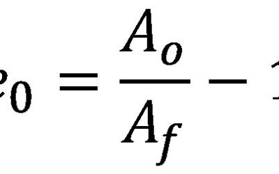
True Fracture Strain
read more