Tensile Testing: Engineering Stress-Strain Curves vs. True Stress-Strain Curves

Tensile Testing: Engineering Stress-Strain Curves vs. True Stress-Strain Curves

Tensile testing is one of the most basic formability characterization methods available.  Results from tensile testing are a key input into metal forming simulations, but if the right information isn’t included, the simulation will not accurately reflect material behavior.   

Metal forming simulation is particularly beneficial on the value-added parts made from advanced high strength steels, since accurate simulations allow for optimal processing with minimal recuts … at least when the right information is used as inputs. 

Engineering illustration of tensile testing comparing engineering strain to tensile strength

Tensile Testing

During tensile testing, a standard sample shape called a dogbone is pulled in tension. Load and displacement are recorded, and which are then converted to a stress-strain curve. Strength is defined as load divided by cross-sectional area. Exactly when the cross-sectional area is measured during the test influences the results.

Before starting the pull, it’s easiest to measure the width and thickness of the test sample.

Engineering drawing (basic) of engineering stress-strain curve

Engineering Stress-Strain Curve

At any load, the engineering stress is the load divided by this initial cross-sectional area. Engineering stress reaches a maximum at the Tensile Strength, which occurs at an engineering strain equal to Uniform Elongation. After that point, engineering stress decreases with increasing strain, progressing until the sample fractures.

However, metals get stronger with deformation through a process known as strain hardening or work hardening. As a tensile test progresses, additional load must be applied to achieve further deformation, even after the “ultimate” tensile strength is reached. Understanding true stress and true strain helps to address the need for additional load after the peak strength is reached.

Illustration with a line chart of true stress-strain curve

During the tensile test, the width and thickness shrink as the length of the test sample increases. Although these dimensional changes are not considered when determining the engineering stress, they are of primary importance when determining true stress. At any load, the true stress is the load divided by the cross-sectional area at that instant.

True Stress-Strain Curve

The true stress – true strain curve gives an accurate view of the stress-strain relationship, one where the stress is not dropping after exceeding the tensile strength stress level.

True stress is determined by dividing the tensile load by the instantaneous area.

True stress-strain curves obtained from tensile bars are valid only through uniform elongation due to the effects of necking and the associated strain state on the calculations. Inaccuracies are introduced if the true stress-true strain curve is extrapolated beyond uniform strain, and as such a different test is needed. Biaxial bulge testing has been used to determine stress-strain curves beyond uniform elongation. Optical measuring systems based on the principles of Digital Image Correlation (DIC) are used to measure strains. The method by which this test is performed is covered in ISO 16808.

Diagram of equation for engineering stress-strain and true stress-strain

Stress-strain curves and associated parameters historically were based on engineering units, since starting dimensions are easily measured and incorporated into the calculations. These are the values you see on certified metal properties, also called metal cert sheets that you get with your steel shipments.

True stress and true strain provide a much better representation of how the material behaves as it is being deformed, which explains its use in computer forming and crash simulations.

It’s much more challenging to get accurate dimensional measurements once the test has started unless there are multiple loops of the operator stopping the test, remeasuring, then restarting the pull. This is not a practical approach.

Fortunately, there are equations that relate engineering units to true units. Conventional stress-strain curves generated in engineering units can be converted to true units for inclusion in simulation software packages.

As the industry moves to more value-added stampings, metal forming simulation is done on nearly every part. The value-added nature of parts made from advanced high strength steels requires best practices be used throughout – otherwise the results from simulation drift further away from matching reality, leading to longer development times and costly recuts.


Danny Schaeffler is the Metallurgy and Forming Technical Editor of the AHSS Applications Guidelines available from WorldAutoSteel. He is founder and President of Engineering Quality Solutions (EQS). Danny wrote the monthly “Science of Forming” and “Metal Matters” column for Metalforming Magazine, and provides seminars on sheet metal formability for Auto/Steel Partnership and the Precision Metalforming Association. He has written for Stamping Journal and The Fabricator, and has lectured at FabTech. Danny is passionate about training new and experienced employees at manufacturing companies about how sheet metal properties impact their forming success.

Uniform Elongation

Uniform Elongation

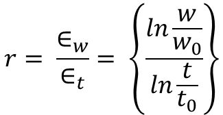
During a tensile test, the elongating sample leads to a reduction in the cross-sectional width and thickness. The shape of the engineering stress-strain curve showing a peak at the load maximum (Figure 1) results from the balance of the work hardening which occurs as metals deform and the reduction in cross-sectional width and thickness which occurs as the sample dogbone is pulled in tension. In the upward sloping region at the beginning of the curve, the effects of work hardening dominate over the cross-sectional reduction. Starting at the load maximum (ultimate tensile strength), the reduction in cross-sectional area of the test sample overpowers the work hardening and the slope of the engineering stress-strain curve decreases. Also beginning at the load maximum, a diffuse neck forms usually in the middle of the sample.

Figure 1: Engineering stress-strain curve from which mechanical properties are derived.

Figure 1: Engineering stress-strain curve from which mechanical properties are derived.


The elongation at which the load maximum occurs is known as Uniform Elongation. In a tensile test, uniform elongation is the percentage the gauge length elongated at peak load relative to the initial gauge length. For example, if the gauge length at peak load measures 61 mm and the initial gauge length was 50mm, uniform elongation is (61-50)/50 = 22%.

Schematics of tensile bar shapes are shown within Figure 1. Note the gauge region highlighted in blue. Up though uniform elongation, the cross-section has a rectangular shape. Necking begins at uniform elongation, and the cross section is no longer rectangular.

Theory and experiments have shown that uniform elongation expressed in true strain units is numerically equivalent to the instantaneous n-value.

Deformation Prior to Uniform Elongation is Not Uniformly Distributed

Conventional wisdom for decades held that there is a uniform distribution of strains within the gauge region of a tensile bar prior to strains reaching uniform elongation. Traditional extensometers calibrated for 50-mm or 80-mm gauge lengths determine elongation from deformation measured relative to this initial length. This approach averages results over these spans.

The advent of Digital Image Correlation (DIC) and advanced processing techniques allowed for a closer look. A studyS-113 released in 2021 clearly showed that each of the 201 data points monitored within a 50 mm gauge length (virtual gauge length of 0.5-mm) experiences a unique strain evolution, with differences starting before uniform elongation.

Figure 2 caption: Strain evolution of the 201 points on the DP980 tensile-test specimen exhibits divergence beginning before uniform elongation—counter to conventional thinking.

Figure 2: Strain evolution of the 201 points on the DP980 tensile-test specimen exhibits divergence beginning before uniform elongation—counter to conventional thinking.S-113


Uniform Elongation

Elastic Modulus

Elastic Modulus (Young’s Modulus)

When a punch initially contacts a sheet metal blank, the forces produced move the sheet metal atoms away from their neutral state and the blank begins to deform. At the atomic level, these forces are called elastic stresses and the deformation is called elastic strain. Forces within the atomic cell are extremely strong: high values of elastic stress results in only small magnitudes of elastic strain. If the force is removed while causing only elastic strain, atoms return to their original lattice position, with no permanent or plastic deformation. The stresses and strains are now at zero.

A stress-strain curve plots stress on the vertical axis, while strain is shown on the horizontal axis (see Figure 2 in Mechanical Properties). At the beginning of this curve, all metals have a characteristic linear relationship between stress and strain. In this linear region, the slope of elastic stress plotted against elastic strain is called the Elastic Modulus or Young’s Modulus or the Modulus of Elasticity, and is typically abbreviated as E. There is a proportional relationship between stress and strain in this section of the stress-strain curve; the strain becomes non-proportional with the onset of plastic (permanent) deformation (see Figure 1).

Figure 1: The Elastic Modulus is the Slope of the Stress-Strain Curve before plastic deformation begins.

Figure 1: The Elastic Modulus is the Slope of the Stress-Strain Curve before plastic deformation begins.


The slope of the modulus line depends on the atomic structure of the metal. Most steels have an atomic unit cell of nine iron atoms – one on each corner of the cube and one in the center of the cube. This is described as a Body Centered Cubic (BCC) structure. The common value for the slope of steel is 210 GPa (30 million psi). In contrast, aluminum and many other non-ferrous metals have 14 atoms as part of the atomic unit cell – one on each corner of the cube and one on each face of the cube. This is referred to as a Face Centered Cubic (FCC) atomic structure. Many aluminum alloys have an elastic modulus of approximately 70 GPa (10 million psi).

Under full press load at bottom dead center, the deformed panel shape is the result of the combination of elastic stress and strain and plastic stress and strain. Removing the forming forces allows the elastic stress and strain to return to zero. The permanent deformation of the sheet metal blank is the formed part coming out of the press, with the release of the elastic stress and strain being the root cause of the detrimental shape phenomenon known as springback. Minimizing or eliminating springback is critical to achieve consistent stamping shape and dimensions.

Depending on panel and process design, some elastic stresses may not be eliminated when the draw panel is removed from the draw press. The elastic stress remaining in the stamping is called residual stress or trapped stress. Any additional change to the stamped panel condition (like trimming, hole punching, bracket welding, reshaping, or other plastic deformation) may change the amount and distribution of residual stresses and therefore potentially change the stamping shape and dimensions.

The amount of springback is inversely proportional to the modulus of elasticity. Therefore, for the same yield stress, steel with three times the modulus of aluminum will have one-third the amount of springback.


Elastic Modulus Variation and Degradation

Analysts often treat the Elastic Modulus as a constant. However, Elastic Modulus varies as a function of orientation relative to the rolling direction (Figure 2). Complicating matters is that this effect changes based on the selected metal grade.

Figure 4:  Modulus of Elasticity as a Function of Orientation for Several Grades (Drawing Steel, DP 590, DP 780, DP 1180, and MS 1700) D-11

Figure 2:  Modulus of Elasticity as a Function of Orientation for Several Grades (Drawing Steel, DP 590, DP 980, DP 1180, and MS 1700) D-11


It is well known that the Bauschinger Effect leads to changes in the Elastic Modulus, and therefore impacts springback. Elastic Modulus determined in the loading portion of the stress-strain curve differs from that determined in the unloading portion. In addition, increasing prestrain lowers the Elastic Modulus, with significant implications for forming and springback simulation accuracy. In DP780, 11% strain resulted in a 28% decrease in the Elastic Modulus, as shown in Figure 3.K-7

Figure 3: Variation of the loading and unloading apparent modulus with strain for DP780K-7

Figure 3: Variation of the loading and unloading apparent modulus with strain for DP780K-7


Another study documented the modulus degradation for many steel grades, including mild steel, conventional high strength steels, and several AHSS products.W-10  Data in some of the grades is limited to small plastic strains, since valid data can be obtained from uniaxial tensile testing only through uniform elongation.  


Reduction in chord modulus for mild steels and conventional high strength steels (left) and for DP and DH steels (right).

Reduction in chord modulus for mild steels and conventional high strength steels (left) and for DP and DH steels (right).W-10


Reduction in chord modulus for CP, CH and MS steels (left) and for a selected of hot rolled steels (right).

Reduction in chord modulus for CP, CH and MS steels (left) and for a selected of hot rolled steels (right).W-10

M-Value

M-Value

M-Value, Strain Rate Sensitivity

The strengthening of some metals changes with the speed at which they are tested. This strain-rate sensitivity is described by the exponent, m, in the modified power law equation:


where έ is the strain rate and m is the strain rate sensitivity.

To characterize the strain rate sensitivity, medium strain rate tests were conducted at strain rates ranging from 10-3/sec (commonly found in tensile tests) to 103/sec. For reference, 101/sec approximates the strain rate observed in a typical stamping. Both yield strength and tensile strength increase with increasing strain rate, as indicated Figures 1 and 2.

Figure 1: Influence of Strain Rate on Yield Strength

Figure 1: Influence of Strain Rate on Yield Strength.Y-1


Figure 2: Influence of Strain Rate on Tensile Strength

Figure 2: Influence of Strain Rate on Tensile Strength.Y-1


Up to a strain rate of 101/sec, both the YS and UTS only increased about 16-20 MPa per order of magnitude increase in strain rate. These increases are less than those measured for low strength steels. This means the YS and UTS values active in the sheet metal are somewhat greater than the reported quasi-static values traditionally reported. However, the change in YS and UTS from small changes in press strokes per minute are very small and are less than the changes experienced from one coil to another.

The change in n-value with increase in strain rate is shown in Figure 3. Steels with YS greater than 300 MPa have an almost constant n-value over the full strain rate range, although some variation from one strain rate to another is possible.

Figure 3: Influence of Strain Rate on n-value

Figure 3: Influence of Strain Rate on n-value.Y-1


Similar behavior was noted in another studyB-22 that included one TRIP steel and three DP steels. Here, DP1000 showed a 50% increase in yield strength when tested at 200/sec compared with conventional tensile test speeds. Strain rate has little influence on the elongation of AHSS at strain rates under 100/sec.

Relationship between strain rate and yield strength (left) and elongation (right)

Figure 4: Relationship between strain rate and yield strength (left) and elongation (right). Citation B-22, as reproduced in Citation D-44


Figure 5 shows the true stress-true strain curves for a processed Press Hardened Steel tested at different strain rates. The yield stress increases approximately five MPa for one order of magnitude increase in strain rate.

Figure 4: True stress-strain curves at different strain rates for 1mm thick Press Hardening Steel (PHS) after heat treatment and quenching.

Figure 5: True stress-strain curves at different strain rates for 1mm thick Press Hardening Steel (PHS) after heat treatment and quenching.V-1


The tensile and fracture response of different grades is a function of the strain rate and cannot be generalized from conventional tensile tests.  This has significant implications when it comes to predicting deformation behavior during the high speeds seen in automotive crash events.  See our page on high speed testing for more details.

Uniform Elongation

Mechanical Properties

Introduction to Mechanical Properties

Tensile property characterization of mild and High Strength Low Alloy steel (HSLA) traditionally was tested only in the rolling direction and included only yield strength, tensile strength, and total elongation. Properties vary as a function of orientation relative to the rolling (grain) direction, so testing in the longitudinal (0°), transverse (90°), and diagonal (45°) orientations relative to the rolling direction is done to obtain a better understanding of metal properties (Figure 1).

A more complete perspective of forming characteristics is obtained by also considering work hardening exponents (n-values) and anisotropy ratios (r-values), both of which are important to achieve improved and consistent formability.

Figure 1. Tensile Test Sample Orientation Relative to Rolling Direction

Figure 1. Tensile Test Sample Orientation Relative to Rolling Direction

Hardness readings are sometimes included in this characterization, but hardness readings are of little use in assessing formability requirements for sheet steel. Hardness testing is best used to assess the heat treatment quality and durability of the tools used to roll, stamp, and cut sheet metal.

The formability limits of different grades of conventional mild and HSLA steels were learned by correlating press performance with as-received mechanical properties. This information can be fed into computer forming simulation packages to run tryouts and troubleshooting in a virtual environment. Many important parameters can be measured in a tensile test, where the output is a stress-strain curve (Figure 2).

Figure 2: Representative Stress-Strain Curve Showing Some Mechanical Properties

Figure 2: Representative Stress-Strain Curve Showing Some Mechanical Properties


Press shop behavior of Advanced High-Strength Steels is more complex. AHSS properties are modified by changing chemistry, annealing temperature, amount of deformation, time, and even deformation path. With new microstructures, these steels become “Designer Steels” with properties tailored not only for initial forming of the stamping but in-service performance requirements for crash resistance, energy absorption, fatigue life, and other needs. An extended list of properties beyond a conventional tensile test is now needed to evaluate total performance with virtual forming prior to cutting the first die, to ensure ordering and receipt of the correct steel, and to enable successful troubleshooting if problems occur.

With increasing use of advanced steels for value-added applications, combined with the natural flow of more manufacturing occurring down the supply chain, it is critical that all levels of suppliers and users understand both how to measure the parameters and how they affect the forming process.


Highlights

    • The multiphase microstructure in Advanced High Strength Steels results in properties that change as the steel is deformed. An in-depth understanding of formability properties is necessary for proper application of these steels.
    • Tensile test data characterizes the ability of a steel grade to perform with respect to global (tensile and necking) formability. Different tests like hole expansion and bending characterize performance at cut edges or bend radii.
    • DP steels have higher n-values in the initial stages of deformation compared to conventional HSLA grades. These higher n-values help distribute deformation more uniformly in the presence of a stress gradient and thereby help minimize strain localization that would otherwise reduce the local thickness of the formed part.
    • The n-value of certain AHSS grades, including dual phase steels, is not constant: there is a higher n-value at lower strains followed by a drop as strain increases.
    • TRIP steels have a smaller initial increase in n-value than DP steels during forming but sustain the increase throughout the entire deformation process. Part designers can use these steels to achieve more complex geometries or further reduce part thickness for weight savings.
    • TRIP steels have retained austenite after forming that transforms into martensite during a crash event, enabling improved crash performance.
    • Normal anisotropy values (rm) approximately equal to 1 are a characteristic of all hot-rolled steels and most cold-rolled and coated AHSS and conventional HSLA steels.
    • AHSS work hardens with increasing strain rate, but the effect is less than observed with mild steel. The n-value changes very little over a 105 (100,000x) increase in strain rate.
    • As-received AHSS does not age-harden in storage.
    • DP and TRIP steels have substantial increase in YS due to a bake hardening effect, while conventional HSLA steels have almost none.
R-Value

R-Value

R-Value, The Plastic Anisotropy Ratio

The r-value, which is also called the Lankford coefficient or the plastic strain ratio, is the ratio of the true width strain to the true thickness strain at a particular value of length strain, indicated in Equation 1. Strains of 15% to 20% are commonly used for determining the r-value of low carbon sheet steel. Like n-value, the ratio will change depending on the chosen reference strain value.


Equation 1


The normal anisotropy ratio (rm) defines the ability of the metal to deform in the thickness direction relative to deformation in the plane of the sheet. rm, also called r-bar (i.e. r average) is the “normal anisotropy parameter” in the formula for Equation 2:


Equation 2


where r0, r90, and r45 are the r-value determined in 0, 90, and 45 degrees relative to the rolling direction.

For rm values greater than one, the sheet metal resists thinning. Values greater than one improve cup drawing (Figure 1), hole expansion, and other forming modes where metal thinning is detrimental. When For rm values are less than one, thinning becomes the preferential metal flow direction, increasing the risk of failure in drawing operations.

Figure 1: Higher r-value is associated with improved deep drawability.

Figure 1: Higher r-value is associated with improved deep drawability.


High-strength steels with tensile strength greater than 450 MPa and hot-rolled steels have rm values close to one. Therefore, conventional HSLA and Advanced High-Strength Steels (AHSS) at similar yield strengths perform equally in forming modes influenced by the rm value. However, r-value for higher strength grades of AHSS (800 MPa or higher) can be lower than one and any performance influenced by r-value would be not as good as HSLA of similar strength. For example, AHSS grades may struggle to form part geometries that require a deep draw, including corners where the steel is under circumferential compression on the binder. This is one of the reasons why higher strength level AHSS grades should have part designs and draw dies developed as “open ended”.

A related parameter is Delta r (∆r), the “planar anisotropy parameter” in the formula shown in Equation 3:


Equation 3


Delta r is an indicator of the ability of a material to demonstrate a non-earing behavior. A value of 0 is ideal in can making or the deep drawing of cylinders, as this indicates equal metal flow in all directions, eliminating the need to trim ears prior to subsequent processing.

Testing procedures for determining r-value are covered in Citations A-44, I-15, J-14.