Press hardening, as we know it today, was developed in Luleå, Sweden, by Norrbottens Järnverks AB (abbreviated as NJA, translated as Norrbotten Iron Works). The first patent application was completed in 1973 and awarded in 1977.N-23 The technology was first commercialized in agriculture components, where the high strength of Press Hardened Steels (PHS) was favored for wear resistance.B-45
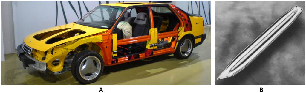
In 1984, automotive applications of PHS started with the Saab 9000 side impact door beams, as seen in Figure 1. A total of 4 parts were used in this car.A-66 The uncoated blanks were almost half the thickness of a cold stamped beam.T-26
Figure 1: Door beams of the Saab 9000 (1984-1998): (a) A see-through car in Saab MuseumS-82, (b) the hot stamped part.L-42
The majority of the PHS parts were door beams through the mid-1990s, with approximately 6 million beams produced in 1996. By this time, the demand for bumper beams was also increasing.F-31 By the end of 1996, the European New Car Assessment Program (EuroNCAP) was formed, which increased the pressure on the OEMs for improved crashworthiness.T-26 In 1998, both the new Volvo S80L-44 and Ford Focus5 were equipped with Press Hardened bumper beams.
The year 1998 saw the development of one of the most important breakthroughs in Press Hardening technology. French steel maker Usinor developed an aluminum-silicon (AlSi) pre-coated steel, commercialized as Usibor 1500 (indicating the typical tensile strength, 1500 MPa.C-24, L-39 In 2000, BMW rolled out its new 3 series convertible. In this vehicle, the A-pillar is made from 3 mm thick uncoated, PHS sheet. This was BMW’s first PHS application, and one of the first PHS A-pillar reinforcement.S-83, S-84 Accra started delivering roll formed PHS components for the Volvo V70, initially an optional 3rd row seating support. Approximately 10,000 parts/year were supplied.G-28
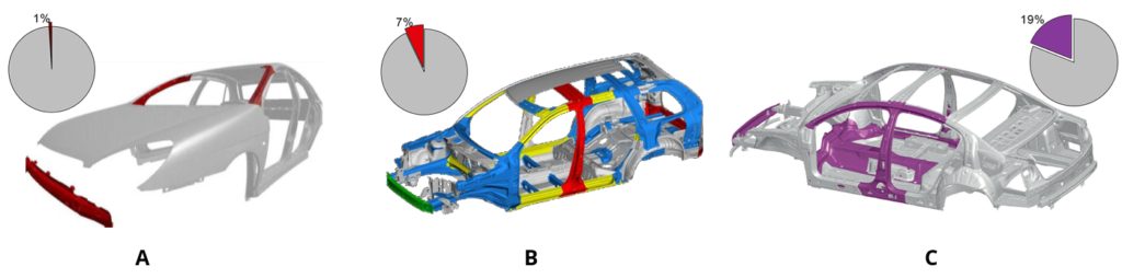
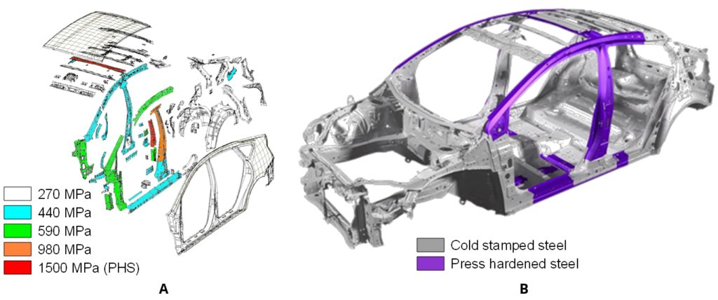
AlSi coated steel was first hot stamped at a French Tier 1 supplier, Sofedit.V-15 This grade was first used in the front bumper beam of the 2nd Generation Renault Laguna (2000-2007). Laguna 2 was the first car to receive a 5-star safety rating from Euro NCAP.V-10 AlSi coated blanks were also used in PSA Group’s Citroën C5 (1st Gen: 2001-2007) in the front bumper beam, and the A-pillars. These three parts weighed a total of 4.5 kg, approximately 1% of the total BIW weight, Figure 2a. About one month later, PSA Group started production of the compact hatchback Peugeot 307, which had five hot stamped components (A- and B-pillars and rear bumper beam). Unlike the Citroën C5, these parts were uncoated. The total weight was 12 kg, corresponding to 3.4% of the BIW weight.R-17, P-27
Volvo started producing the XC90 SUV in 2002. The body-in-white with doors and closures weighed 531 kg.B-44 A total of 10 parts, weighing 37 kg are either roll formed or direct stamped PHS. This accounts for approximately 7% of the BIW weight.L-43 During its time, this was the highest use of PHS in car bodies. In Figure 2b, the Press Hardened components other than the 2nd row seat frame, which is a load bearing body part, are shown.
Accelerated Use and Globalization
The use of press hardened parts increased rapidly after the introduction of the VW Passat in 2005. This car had approximately 19% of its BIW (by weight) made from press hardened steels, Figure 2c. Some parts in this car saw the first use of varnish coated blanks in a two-step hybrid process. Three parts were produced using either an indirect or hybrid process, including the transmission tunnel.H-50
Following are a few highlights of PHS use in vehicle applications during this time period :
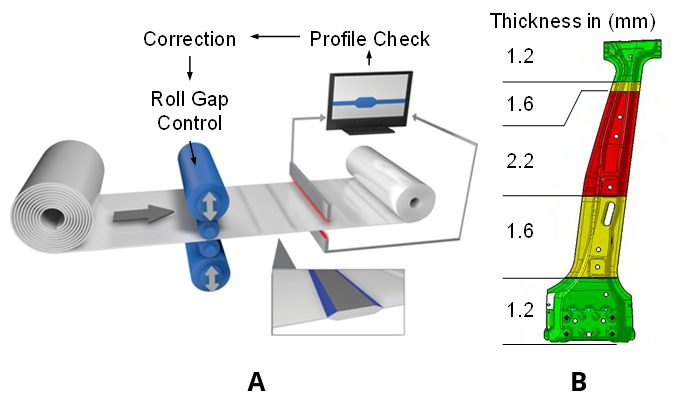
In 2006, the Dodge CaliberK-37 and BMW X5P-28 were among the first cars to have tailor-rolled and Press Hardened components in their bodies (Figure 3).
Figure 3: (a) Tailor Rolling ProcessZ-5, (b) B-pillar of BMW X5 (2nd Gen: 2006-2013).P-28
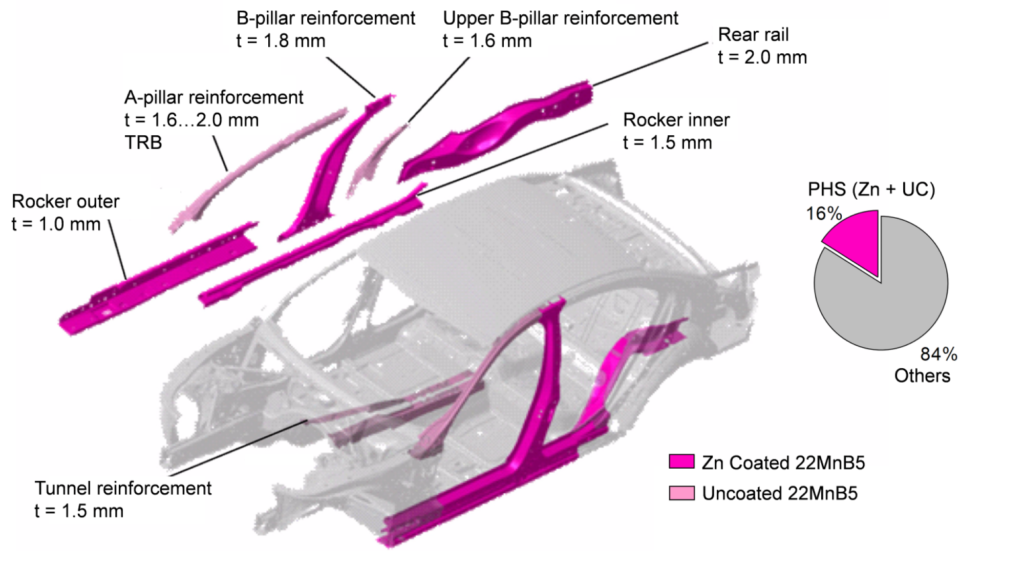
BMW 7 Series (5th Gen: 2008-2015) became the first car to have Zn-coated Press Hardened components in its body-in-white. The car also contained uncoated parts, as shown in Figure 4 (next page). The total PHS usage in this car was approximately 16%.P-20
Figure 4: PHS usage in BMW 7 Series (5th Gen: 2008-2015) (re-created using P-20).
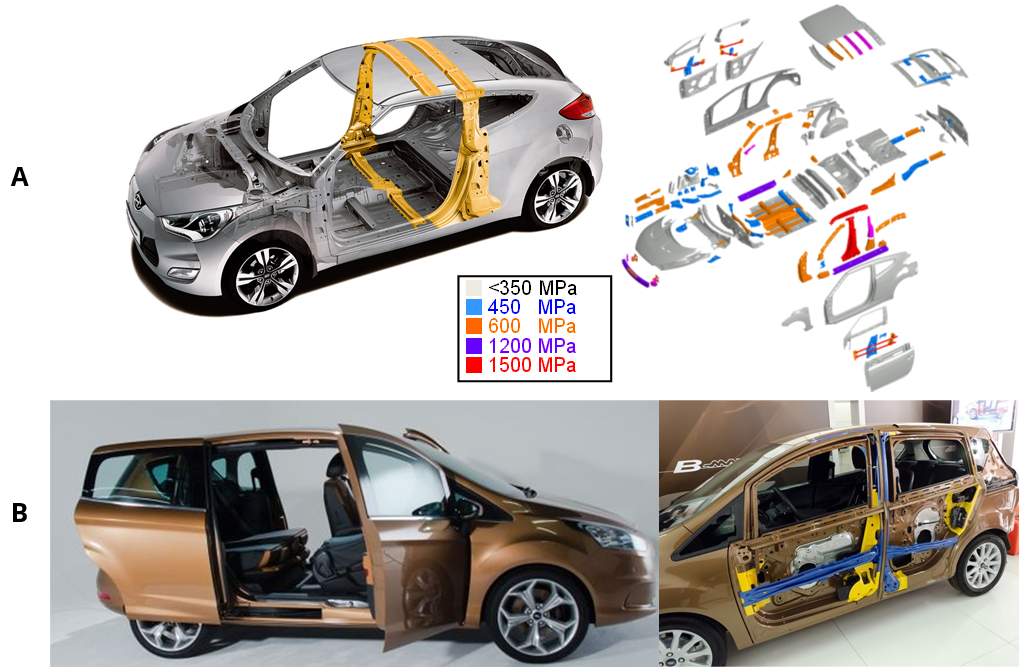
Press hardening also allowed car makers to create unconventional cars. In 2011, Hyundai rolled out the 1st generation Veloster, a 3-door coupé (also known as 2+1, with one door on the driver side and 2 doors on the passenger side), and as such containing axisymmetric front doors. Thus, the car could not have a full B-ring, as illustrated in Figure 5a.B-14, R-19 Another unconventional design was the Ford B-Max subcompact MPV sold in Europe between 2012 and 2017. The car had conventional swing doors in the front and two sliding rear doors. A PHS B-pillar was integrated in the doors, providing ease of ingress. Its PHS components (integrated B-pillar in front and rear doors, door beams and cantrail) are shown with blue color in Figure 5b.B-14, L-45
Figure 5: Unconventional car designs with PHS: (a) Hyundai Veloster, asymmetric 2+1 doors coupé (re-created after Citation R-19), and (b) Ford B-Max, sub-compact MPV with integrated B-pillars in the doors.L-45
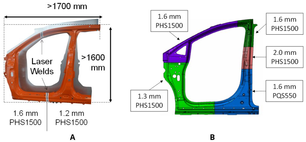
In 2013, the Acura MDX (3rd Gen: 2013-2020) became the first car to have a Hot Stamped door ring. The part was a tailor welded blank comprised of two sub-blanks, as shown in Figure 6a. The design saved about 6.2 kg weight per car and had high material utilization ratio thanks to sub-blank nesting optimization.A-67, M-46One of the most recent PHS applications was in 2017 Chrysler Pacifica with 5 sub-blanks, as shown in Figure 6b. This car also has a PQS550 sub-blank at the lower B-pillar region.D-28
Figure 6: Hot stamped door rings: (a) First application in 2013 Acura MDX had 2 sub-blanks, (b) a more recent application in 2017 Chrysler Pacifica has five sub-blanks with PQS550 at the lower B-pillar (re-created after Citations B-14, A-67, D-28).
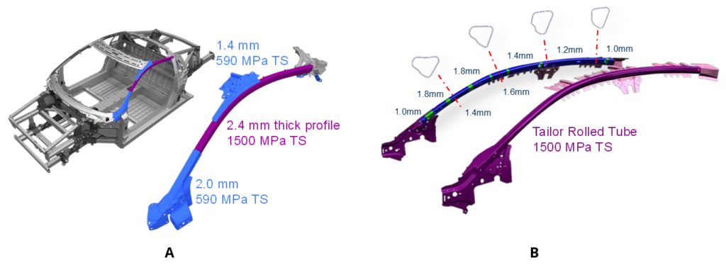
Tubular hardened steels have been long used in car bodies, with minimal forming. Since 2013, a special 3-D hot bending and quenching (3DQ) process has been employed. One of the earliest uses of this technology was Mazda Premacy (known as Mazda 5 in some markets). The same process was also used in making the A-pillars of the Acura NSX (Honda NSX in some markets, 2016-present), as seen in Figure 7a.H-29 Since 2018, tubular parts formed with internal pressure, called form blow hardened parts, are used in the Ford Focus (4th Generation) (Figure 7b) and Jeep Wrangler (4th Generation).B-16, B-17
Figure 7: Tubular hardened steel usage in A-pillars of: (a) 2015 Acura NSXH-29, (b) 2018 Ford Focus.B-16
PHS Use in xEVs: Hybrid Electric, Battery Electric,
Plug-in Hybrid Electric & Fuel Cell Electric Vehicles
The first commercially available Hybrid Electric Vehicle (HEV) was the Toyota Prius (1st Gen: 1997-2003). The second-generation Prius (2003-2009) had very few Press Hardened components, as shown with red color in Figure 8a. This was the first time Toyota used hot stamped components.M-47 The third generation Prius (2009-2015) had approximately 3% of its BIW Press Hardened. In the 4th generation Prius released in 2015, the share of >980 MPa steels has risen to 19%.U-10 Figure 8b shows the Press Hardened parts in this latest Prius.K-38
Figure 8: PHS usage in Toyota Prius: (a) 2nd generation (2003-2009) and (b) 4th generation (2015-present) (re-created after Citations M-47 and K-38)
The 2012 Tesla Model S and Model X launched using aluminium bodies, with PHS reinforcements in the pillars and the bumpers. Model S is known to have a roll-formed PHS bumper beam. High volume Model 3 and Model Y have a significant amount of press hardened components in their bodies.T-35
In 2011, General Motors started production of its first Plug-in Hybrid Electric Vehicle (PHEV), the Chevrolet Volt (known as Opel Ampera in EU and Vauxhall Ampera in the UK). This car had six Hot Stamped components, including A and B pillars, accounting for slightly over 5% of the BIW mass.P-29
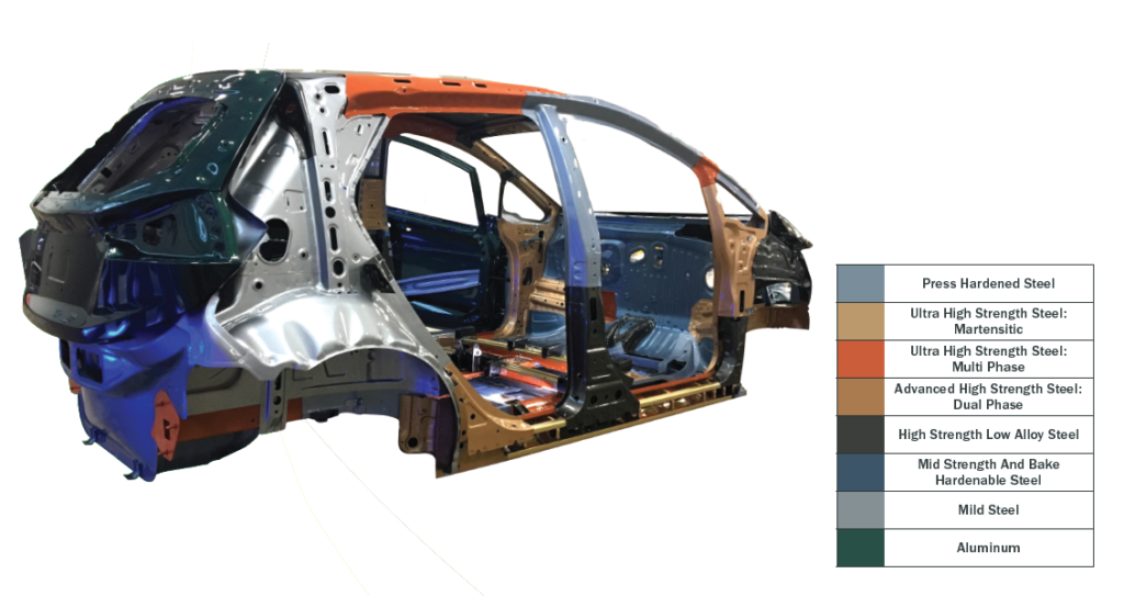
The smaller BEV Chevrolet Bolt, launched in 2017, had aluminum closures, but a steel-intensive BIW that is 80% steel, 44% of which is Advanced High-Strength Steels including 11.8% PHS. Figure 9.A-69
Figure 9: Chevrolet Bolt Body Structure and Steel Content.A-69
In December 2020, Hyundai announced their new electric platform, E-GMP. The platform will utilize Press Hardened steel components to secure the batteries.H-52
Automakers have turned to PHS to manage the extra load of Fuel Cell powertrains as well. The first-generation Toyota Mirai had only Press Hardened B-pillars, cantrails and lateral floor members.T-38 The second generation has a number of parts with PHS in its under body as well.T-39
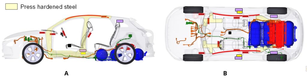
In 2018, Hyundai Nexo became the first fuel-cell car to be tested by EuroNCAP, achieving a 5-Star rating. The car has PHS A- and B-pillars, rocker reinforcements, and several under body components, as seen in Figure 10.H-53
Figure 10: Press hardened steel usage in Hyundai Nexo Fuel Cell vehicle: (a) side view and (b) top view (re-created after Citation H-53).
Multi-phase steels are complex to cut and form, requiring specific tooling materials. The tooling alloys which have been used for decades, such as D2, A2 or S7, are reaching their load limits and often result in unacceptable tool life. The mechanical properties of the sheet steels achieve tensile strengths of up to 1800 MPa with elongations of up to 40%. Additionally, the tooling alloys are stressed by the work hardening of the material during processing.
The challenge to process AHSS quickly and economically makes it necessary for suppliers to manufacture tooling with an optimal tool steel selection. The following case study illustrates the tooling challenges caused by AHSS and the importance of proper tool steel selection.
A manufacturer of control arms changed production material from a conventional steel to an Advanced High-Strength Steel (AHSS), HR440Y580T-FB, a Ferrite-Bainite grade with a minimum yield strength of 440 MPa and a minimum tensile strength of 580 MPa. However, the tool steels were not also changed to address the increased demands of AHSS, resulting in unacceptable tool life and down time.
According to the certified metal properties, the 4 mm thick FB 600 material introduced into production had a 525 MPa yield strength, 605 MPa tensile strength, and a 20% total elongation. These mechanical properties did not appear to be a significant challenge for the tool steels specified in the existing die standards. But the problems encountered in production revealed serious tool life problems.
To form the FB 600 the manufacturer used D2 steel. D2 was successful for decades in forming applications. This cold work tool steel is used in a wide variety of applications due to its simple heat treatment and its easily adjustable hardness values. In this case, D2 was used at a hardness of RC 58/60.
While tools manufactured from D2 can withstand up to 50,000 load cycles when forming conventional steels, these particular D2 tools failed after only 5,000 – 7,000 cycles during the forming of FB 600. The first problems were detected on a curl station where mechanical overload caused the D2 tools to break catastrophically, as seen in Figure 1 below. Since the breakage was sudden and unforeseeable, each failure of the tools resulted in long changeover times and thus machine downtime.
Figure 9: Breakage seen in control arm curl tool made from D2, leading to premature failure. Conversion to a PM tool steel having higher impact resistance led to 10x increase in tool life.M-20
Since the cause of failure was a mechanical breakage of the tools, a tougher alternative was consequently sought. These alternatives, which included A2 and DC53 were tested at RC 58-60 and unfortunately showed similar tool life and failures.
Metallurgical analysis indicated that the failure resulted from insufficient impact strength of the tool steel. This was caused by the increased cross-cut that the work-hardened AHSS exerted on the curl. As an alternative material, a cold work steel with a hardness of 58-60, a tensile strength of about 2200 – 2400 MPa and high toughness was sought. These properties could not be achieved with conventional tool steels. The toolmaker used a special particle metallurgy (PM) tool steel to obtain an optimum combination of impact strength, hardness and wear resistance.
Particle metallurgy (PM) tool steels, due to their unique manufacturing process, represent improvements in alloy composition beyond the capabilities of conventional tool steels. Materials with a high alloy content of carbide formers such as chromium, vanadium, molybdenum and tungsten are readily available. The PM melting process ensures that the carbides are especially fine in particle size and evenly distributed (reference Table 1). This process results in a far tougher tool steel compared to conventional melting practices.
Table 1: Elemental Composition of Chosen Tool Steel
The manufacturer selected Z-Tuff PM® to be used at a hardness of RC 58-60. Employing the identical hardness as the conventional cold work steel D2, a significant increase in impact strength (nearly 10X increase as measured by un-notched Charpy impact values) was realized due to the homogeneous microstructure and the more evenly distributed precipitates. This positive effect of the PM material led to a significant increase in tool life. By switching to the PM tool steel, the service life is again at the usual 40000 – 50000 load cycles. By using a steel with an optimal combination of properties, the manufacturer eliminated the tool breakage without introducing new problems such as deformation, galling, or premature wear.
AHSS creates tooling demands that challenge the mechanical properties of conventional tool steels. Existing die standards may not be sufficient to achieve consistent and reliable performance for forming, trimming and piercing AHSS. Proper tool steel grade selection is critical to ensuring consistent and reliable tooling performance in AHSS applications. Powder metallurgical tool steels offer a solution for the challenges of AHSS.
A New Software Application for Thin Wall Section Analysis
Advanced High-Strength Steel (AHSS) grades offer increased performance in yield and tensile strength. However, to fully utilize this increased strength, automotive beam sections must be designed carefully to avoid buckling of the plate elements in the section. A new software application, Geometric Analysis of Sections—GAS2.0, available through the American Iron and Steel Institute, is a tool to aid in this design effort.
Plate Buckling in Automotive Sections
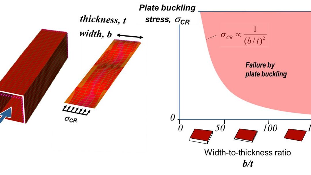
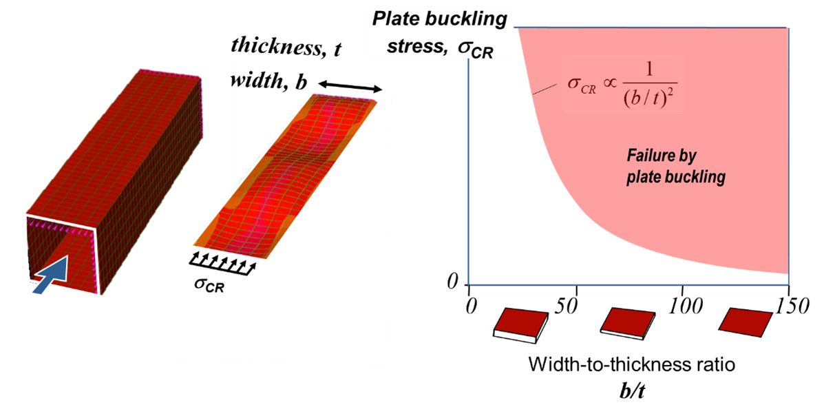
To understand how plate buckling affects the strength of a thin walled beam consider Figure 1. A square beam is made of four identical plates connected at their edges. Under an axial compressive load each plate may buckle. Considering just one of the plates, the stress that will cause buckling depends on the ratio of plate width and thickness (b/t). Thinner wider plates with large b/t ratio will buckle at a lower stress than thicker narrower plates.
Figure 1: Plate Buckling Behavior.
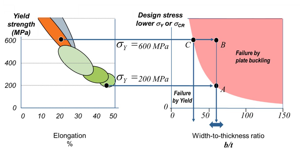
Now consider a plate of mild steel (200 MPa yield stress) which has been designed to buckle just as yield stress is reached, Point A in Figure 2. The plate would have a b/t ratio of approximately 60. This design is taking full advantage of the yield strength of the material.
Now consider the same plate but substituting an AHSS grade (600 MPa yield stress) as shown in Figure 2. The plate will buckle at the same 200 MPa before reaching the material’s potential, Point B in the figure. To take advantage of this materials yield strength, the proportions of the plate will need to be changed, Point C. This illustration demonstrates the need to consider plate buckling particularly in the application of AHSS grades.
Figure 2: AHSS Substitution in a Plate.
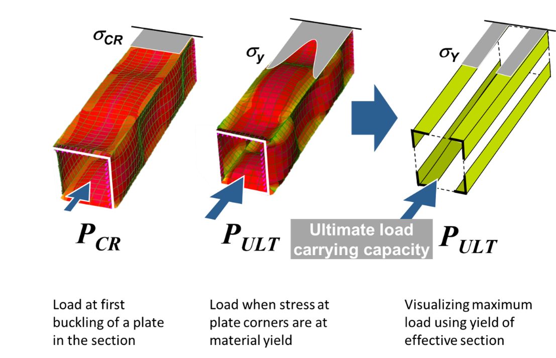
Moving from a single plate to the more complex case of a beam section of several plates, consider Figure 3. On the left is the beam made of four plates with a compressive load causing the plates to just begin to buckle. However, this condition does not represent the maximum load carrying ability of the beam. The load can be increased until the stress at the corners of the buckled plates are at the material yield stress, center in Figure 3. Note that in this condition the stress distribution across the plate is nonlinear with lower stress in the center of each plate. One means to model this complex state is by using an imaginary Effective Section. Here the center portion is visualized as being removed and the remainder of the section is stressed uniformly at yield. The amount of plate width to be removed is determined by theory.W-21, A-42, Y-9, M-18 The effective section is a convenient way to visualize the efficiency of a section design given the material grade and provides an estimate of the maximum load carrying ability of the beam.
Figure 3: Concept of Effective Section.
Geometric Analysis of Sections – GAS2.0
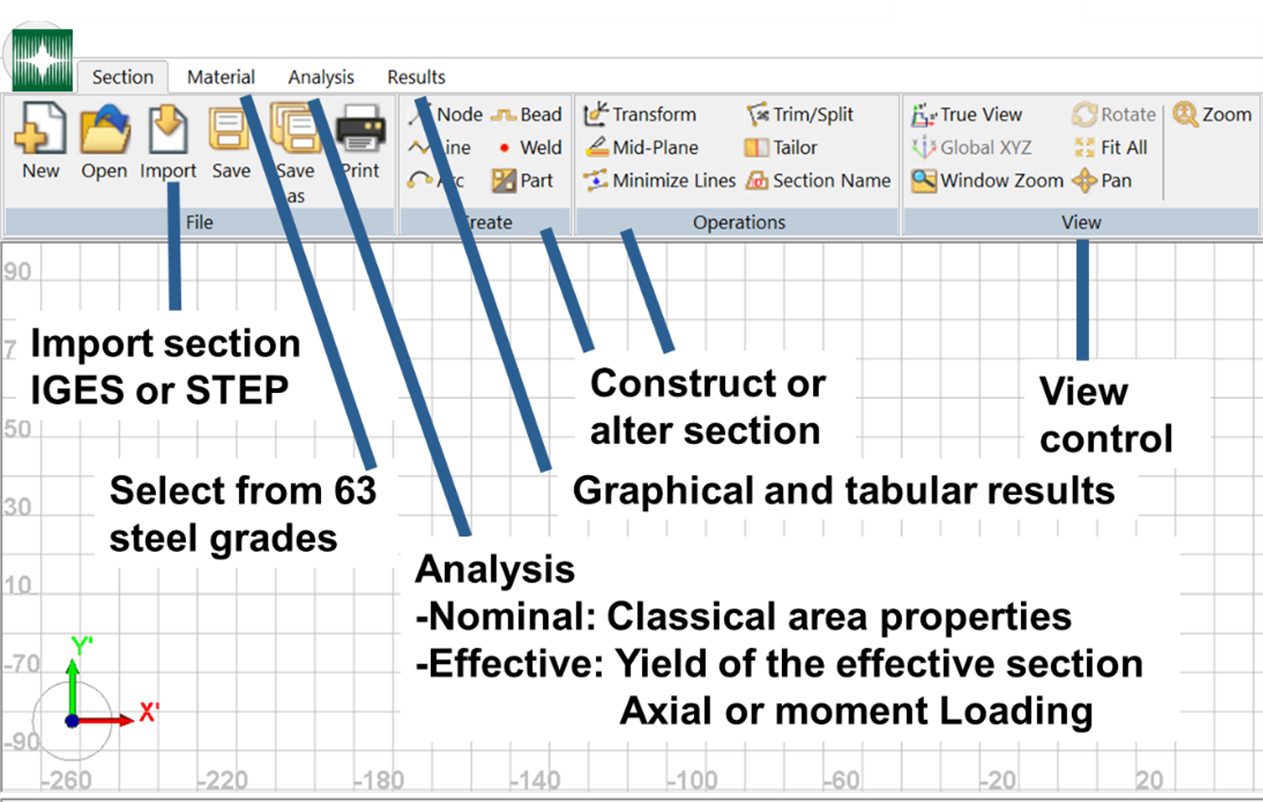
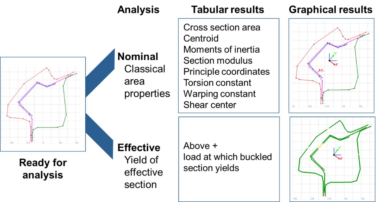
Geometrical Analysis of Sections software determines the effective section for complex automotive sections. Figure 4 illustrates the GAS2.0 user interface. The user has the ability to construct sections or to import section data from a CAD system. Material properties for 63 steel grades are preloaded with the ability to also add user-defined steel grades. Two types of analysis are available. Nominal analysis, which provides classical area properties of the section, and Effective analysis which determines the effective section at material yield. Figure 5 summarizes both the tabular results and graphical results for each type of analysis.
Figure 4: GAS2.0 User Interface.
Figure 5. GAS2.0 Analysis Results.
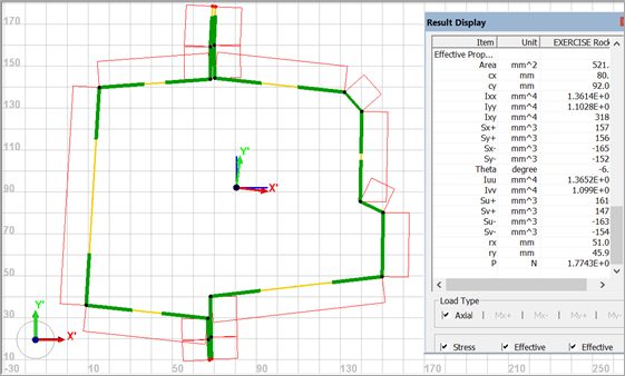
Figure 6 illustrates an example of an Effective Analysis for a rocker section. In the graphical screen, the effective section is shown in green. Ideally, the whole section would be effective to fully use the materials yield capability. Also shown in the graphical screen are the section centroid, orientation of the principle coordinates, and stress distribution. In the right text box are tabular results. At the bottom of the tabular results is the axial load that causes this stress state and represents the ultimate load carrying ability of this section.
Figure 6: GAS2.0 Graphical Results.
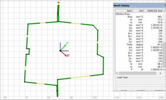
It is clear that much of the material in the section of Figure 6 is not fully effective. GAS2.0 allows the user to conveniently modify the section. For example, in Figure 7 a bead has been added to the left side wall increasing its bulking resistance. Note that the side wall is now largely effective, and the ultimate load at the bottom of the text box has increased substantially.
Figure 7: Improved Design Concept.
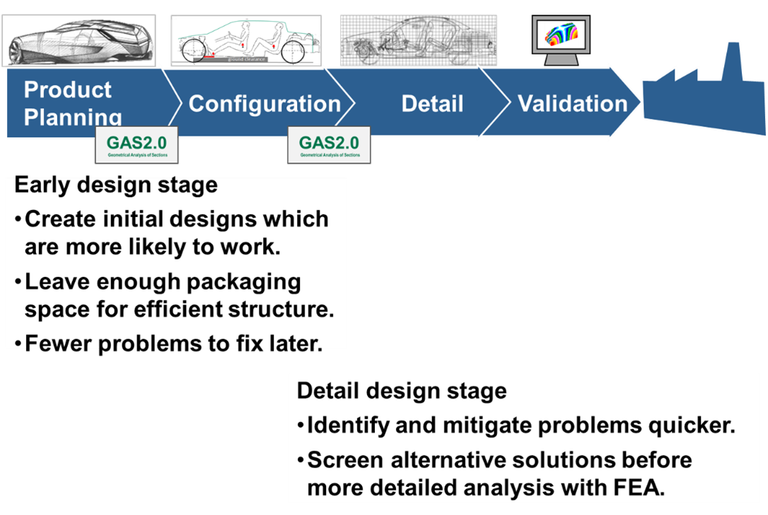
Role of GAS in the Design Process
GAS2.0 can play a significant role in early stage design, see Figure 8, by quickly creating initial designs which are more likely to function and to ensure that adequate package space is set aside for structure. This will result in fewer problems to fix later in the design sequence. During the detail design stage, GAS2.0 can supplement Finite Element Analysis by identifying problems earlier, and by screening design concepts for those with the greatest promise prior to more detailed analysis by FEA.
Figure 8: Role of GAS2.0 in Design Process.
GAS2.0 is available for free download at www.steel.org, Included in the resources at steel.org is an American Iron and Steel Institute introductory webinar conducted by Dr. Don Malen on 16 June 2020, as well as a number of GAS2.0 tutorials and training modules.
You are most likely wondering why WorldAutoSteel is writing a blog about a bicycle. It is because when we talked to Jia-Uei Chan, Regional Business Development at our member company, thyssenkrupp Steel Europe (TKSe), about the journey of inventing the world’s first Advanced High-Strength Steel road bike, we were incredibly inspired. This is more than a story about a steel bicycle. This is the story of steel innovation, conceived in a WorldAutoSteel members workshop to brainstorm ideas on transforming steel’s image to the sophisticated and advanced material it is. Their journey led to new steel applications, patentable processes, and in the steelworks bicycle, ideas that we think can inspire new automotive applications as well. And anyway, who doesn’t like an inspiring story?
Bikes of this genre have some of the same requirements of modern vehicles: lightweight, strength and durability, affordability, and high performance. To achieve these, the thyssenkrupp steelworks team developed what they called inbike® technology, which combines high-strength steel, half-shell technology and automated laser welding.
How it was made
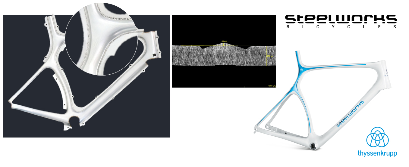
The bike frame is made from DP 330/590 steel, used for its cold forming abilities, stamped as thin as 0.7mm. The steel blanks are pressed into a die to form two half-shells in a deep-drawing process.
A major challenge was to bring these two half shells together in such a way that minimized gaps and achieved a tight fit, enabling automated laser welding (this process requires no gaps over 6 meters of contact length), while ensuring that the frame achieves an elegant, seamless look. Enter innovation.
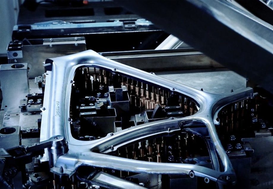
At the stamping plant, the half-shells were fitted with “dimples,” (See Figure 1) tiny bumps on the welding flanges that create channels at the weld seam for the zinc, preventing vaporized zinc from remaining trapped in the seam during subsequent welding. The half shells were then clamped in a special device and shipped to the laser specialist (See Figure 2).
Figure 1: Tiny bumps prevent vaporized zinc from remaining trapped in the seam during subsequent welding.
Figure 2: Frame half-shells clamped in the device for laser welding.
The particular challenge lay in the reliable processing and fusing of both frame halves by means of automated laser welding in such a way that no damage to the frame would occur, while also ensuring the weld seam lay as close as possible to the bend radius of the frame halves. The complex frame shape is welded by following a sophisticated trajectory in a 3-D space. After countless continuous improvement exercises, the steelworks team was able to achieve a very flat, elegant weld seam design. This translates into a very stable bike, with a frame that has the needed rigidity in the bottom bracket area to enable high biomechanical power transmission, but with high elasticity in the seat tube configuration to make for an unusually comfortable ride. In comparison, aluminium and carbon fiber bikes are very stiff and characteristic of an unpleasant ride experience.
Inventing the possibility
Tackling a project that is such a reach beyond the norm is never easy. The thyssenkrupp steelworks team repeatedly heard from qualified experts that the project was actually not feasible. At the same time, they had partners who were so fascinated by the challenge that they wanted to make it possible. Chan related to WorldAutoSteel that there were many times when giving up was the more attractive option. Endurance won out. And as it turns out, the half-shell technology invented out of necessity for this bike could find an application in the tough requirements of an electric vehicle battery case.
Says Chan, “We genuinely believed that steel is the perfect material for a road bike. And we wanted to break with convention and make the most out of steel with high-tech engineering.” Have a look at steelworks.bike, and you will undoubtedly agree they did just that.
Dr. Donald Malen, College of Engineering, University of Michigan, reviews the use of two recently developed Powertrain Models, which he co-authored with Dr. Roland Geyer, University of California, Bren School of Environmental Science.
The use of Advanced High-Strength Steel (AHSS) grades offer a means to lightweight a vehicle. Among the benefits of this lightweighting are less fuel used over the vehicle life, and better acceleration performance. Vehicle designers as well as Greenhouse Gas analysts are interested in estimating these benefits early in the vehicle design process. G-13
Models are constructed for this purpose which range from the use of a simple coefficient, (for example fuel consumption change per kg of mass reduction), to very detailed models accessible only to specialists which require knowledge of hundreds of vehicle parameters. Draw backs to the first approach is that the coefficient may be based on assumptions about the vehicle which do not match the current case. Drawbacks to the detailed models are the considerable expense and time needed, and the lack of transparency in the results; It is difficult to relate inputs with outputs.
A middle way between the simplistic coefficient and the complex model, is described here as a set of Parsimonious Powertrain Models. G-10, G-11, G-12 Parsimony is the principle that the best model is the one that requires the fewest assumptions while still providing adequate estimates. These Excel spreadsheet models cover Internal Combustion powertrains, Battery Electric Vehicles, and Plug-in Electric Vehicles, and predict fuel consumption and acceleration performance based on a small set of inputs. Inputs include vehicle characteristics (mass, drag coefficient, frontal area, rolling resistance), powertrain characteristics (fuel conversion efficiency, gear ratios, gear train efficiency), and fuel consumption driving cycle. Model outputs include estimates for fuel consumption, acceleration, and a visitation map.
Physics of the Models
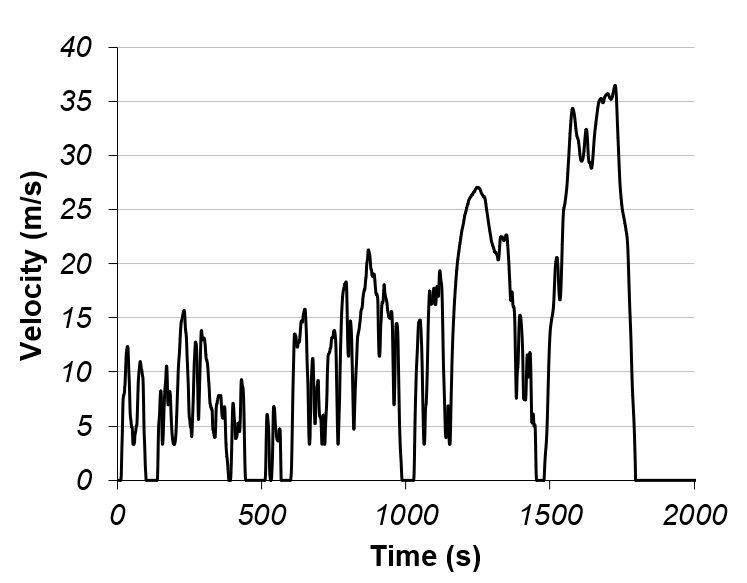
Fuel consumption is determined by the quantity of fuel used over a driving cycle. The driving cycle specifies the vehicle speed vs. time. An example of a driving cycle is the World Light Vehicles Test Procedure (WLTP) cycle shown in Figure 1.
Figure 1: Fuel Consumption Driving Cycle (WLTP Class 3b).
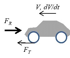
Given the velocity history of Figure 1, the forces on the vehicle resisting forward motion may be calculated. These forces include inertia force, aerodynamic drag force, and rolling resistance. The total of these forces, called tractive force, must be provided by the vehicle propulsion system, see Figure 2.
Figure 2. Tractive Force Required.
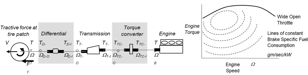
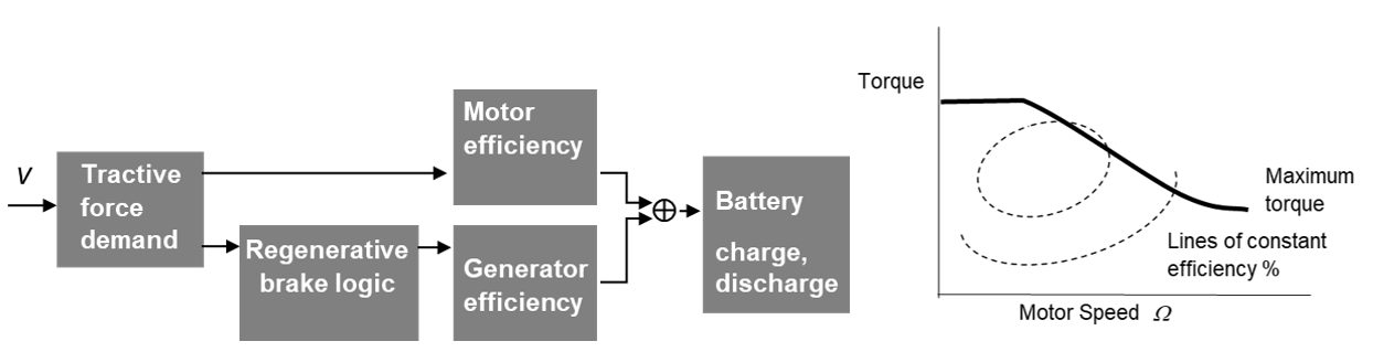
Once vehicle speed and tractive force are known at each point of time during the driving cycle, the required torque and rotational speed may be determined for each of the drivetrain elements, as shown in Figure 3 for an Internal Combustion system, and Figure 4 for a Battery Electric Vehicle.
Figure 3. Internal Combustion Powertrain.
Figure 4. Battery Electric Vehicle Powertrain.
In this way, the required torque and speed of the engine or motor may be determined. Then using a map of efficiency, shown to the right in Figures 3 and 4, the energy demand is determined at each point in time. Summing the energy demand over time yields the fuel used over the driving cycle. The reader is referred to References 1 and 2 for a much more in depth description of the models.
Example Application
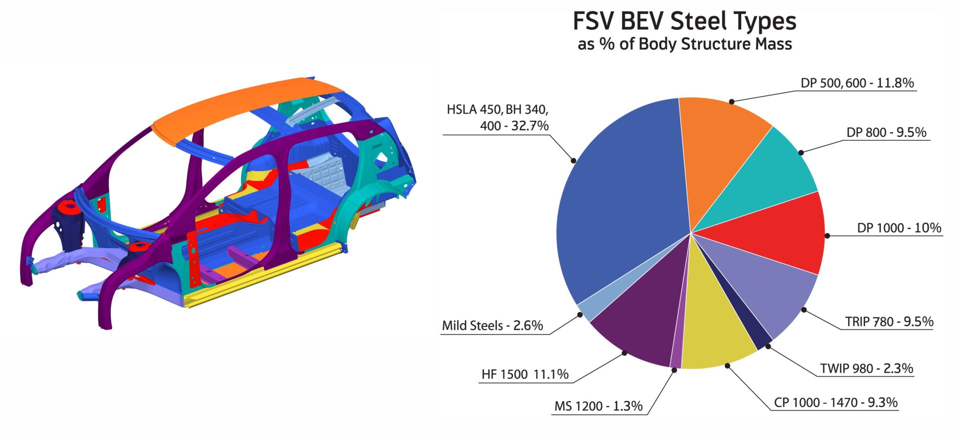
As an example application, consider the WorldAutoSteel FutureSteelVehicle (FSV).W-7 The FSV project, completed in 2011, investigated the weight reduction potential enabled with the use of AHSS, advanced manufacturing processes and computer optimization. The resulting material use in the body structure is shown in Figure 5.
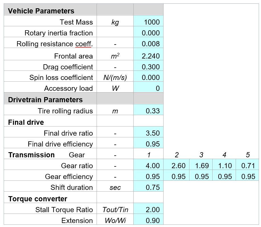
This use of AHSS allowed a reduction in the vehicle curb mass from 1200 kg to 1000 kg. What are the effects of this mass reduction on fuel consumption and acceleration performance? The inputs required for the powertrain model are shown in Table 1 for the base case.
Table 1: Model Inputs for Base Case.
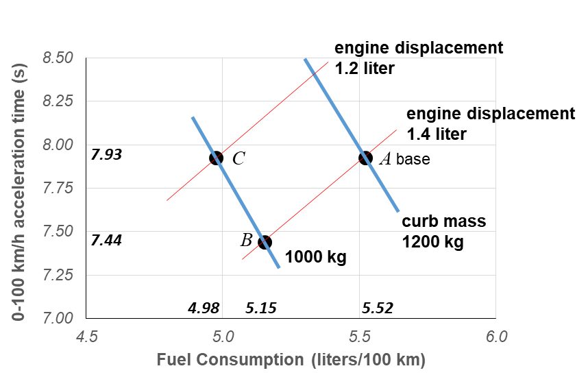
The results provided by the powertrain model are summarized in the acceleration-time vs. fuel consumption graph of Figure 6. Point A is the base case at 1200 kg curb mass. The lightweight case with same engine is shown as Point B. Note the fuel consumption reduction and also the acceleration time reduction. Often the acceleration time is set as a requirement. For the lighter vehicle, the engine size may be reduced to achieve the original acceleration time and an even greater reduction in fuel consumption as shown as Point C.
Figure 6. Summary of results of base vehicle and reduced mass vehicle.
Using the parsimonious powertrain models allows such ‘what-if’ questions to be answered quickly, with minimal data input, and in a transparent way. The Parsimonious Powertrain Models are available as a free download at worldautosteel.org.
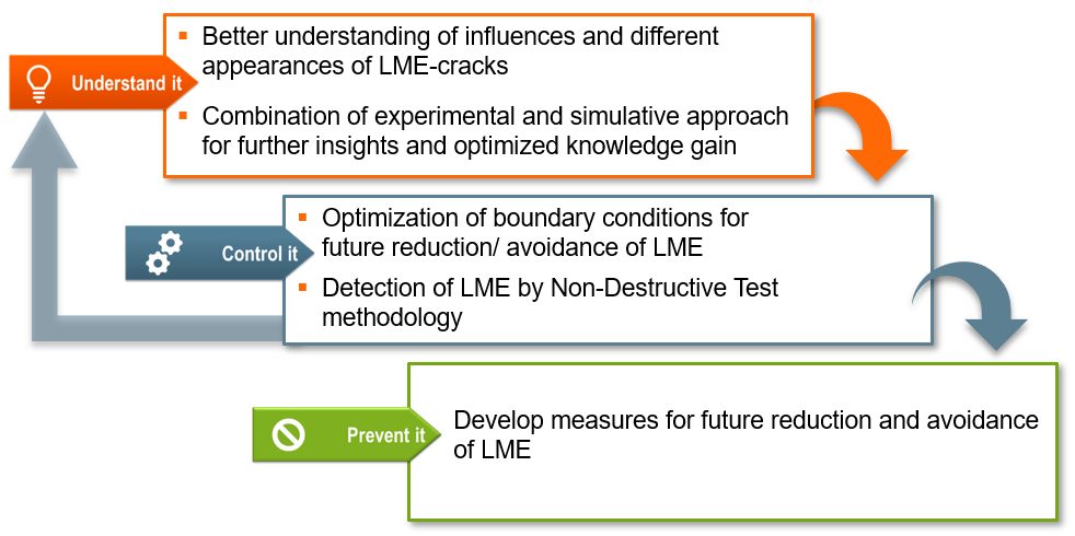
WorldAutoSteel releases today the results of a three-year study on Liquid Metal Embrittlement (LME), a type of cracking that is reported to occur in the welding of Advanced High-Strength Steels (AHSS).The study results add important knowledge and data to understanding the mechanisms behind LME and thereby finding methods to control and establish parameters for preventing its occurrence. As well, the study investigated possible consequences of residual LME on part performance, as well as non-destructive methods for detecting and characterizing LME cracking, both in the laboratory and on the manufacturing line (Figure 1).
Figure 1: LME Study Scope
The study encompassed three different research fields, with an expert institute engaged for each:
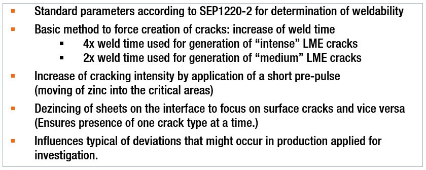
A portfolio containing 13 anonymized AHSS grades, including dual phase (DP), martensitic (MS) and retained austenite (RA) with an ultimate tensile strength (UTS) of 800 MPa and higher, was used to set up a testing matrix, which enabled the replication of the most relevant and critical material thickness combinations (MTC). All considered MTCs show a sufficient weldability under use of standard parameters according to SEP1220-2. Additional MTCs included the joining of various strengths and thicknesses of mild steels to select AHSS in the portfolio. Figure 2 provides the welding parameters used throughout the study.
Figure 2: Study Welding Parameters
In parallel, a 3D electro-thermomechanical simulation model was set up to study LME. The model is based on temperature-dependent material data for dual phase AHSS as well as electrical and thermal contact resistance measurements and calculates local heating due to current flow as well as mechanical stresses and strains. It proved particularly useful in providing additional means to mathematically study the dynamics observed in the experimental tests. This model development was documented in two previous AHSS Insights blogs (see AHSS Insights Related Articles below).
Understanding LME
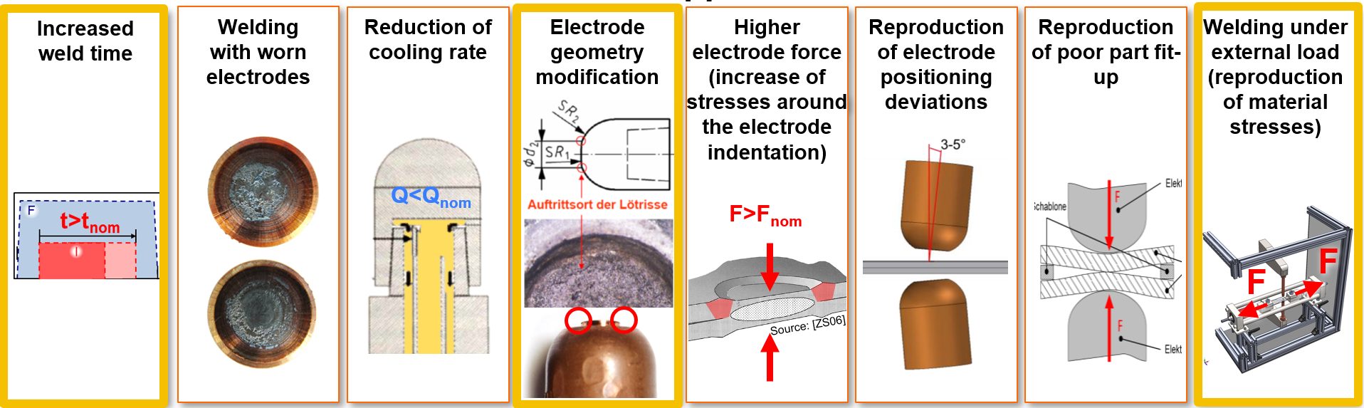
The study began by analyzing different influence factors (Figure 3) which resembled typical process deviations that might occur during car body production. The impact of the influences was analyzed by the degree of cracking observed for each factor. A select number of welding set-ups from these investigations were rebuilt digitally in the simulation model to replicate the process and study its dynamics mathematically. This further enabled the clarification of important cause-effect relationships.
Figure 3: Overview of All Applied Influence Factors (those outlined in yellow resulted in most frequent cracking.)
Generally, the most frequent cracking was observed for sharp electrode geometries, increased weld times and application of external loads during welding. All three factors were closely analyzed by combining the experimental approach with the numerical approach using the simulation model.
Destructive Testing – LME Effects on Mechanical Joint Strength
A destructive testing program also was conducted for an evaluation of LME impact on mechanical joint strength and load bearing capacity in multiple conditions, including quasi-static loading, cyclic loading, crash tests and corrosion. In summary of all load cases, it can be concluded that LME cracks, which might be caused by typical process deviations (e.g. bad part fit up, worn electrodes) have a low intensity impact and do not affect the mechanical strength of the spot weld. And as previously mentioned, the study analyses showed that a complete avoidance of LME during resistance spot welding is possible by the application of measures for reducing the critical conditions from local strains and exposure to liquid zinc.
Controlling LME
In welding under external load experiments, the locations of the experimental crack occurrence showed close correlation with the strains and remaining plastic deformations computed by the simulation model. It was observed that the cracks form at the location of the highest plastic strains, and material-specific threshold values for critical strains were derived. The threshold values then were used to judge the crack formation at elongated weld times.
At the same time, the simulation model pointed out a significant difference in liquid zinc diffusion during elongated weld times. Therefore, it is concluded that liquid zinc exposure time is a second highly relevant factor for LME formation.
The results for the remaining influence factors depended on the investigated MTCs and were generally less significant. In more susceptible MTCs (AHSS welded with thick Mild steel), no significant cracking occurred when welded using standard process parameters. Light cracking was observed for most of the investigated influences, such as low electrode cooling rate, worn electrode caps, electrode positioning deviations or for gap afflicted spot welds. More intense cracking (higher penetration depth cracking) was only observed when welding under extremely high external loads (0.8 Re) or, even more, as a consequence of highly increased weld times.
For the non-susceptible MTCs, even extreme situations and weld set-ups (such as the described elongated weld times) did not result in significant LME cracks within the investigated AHSS grades.
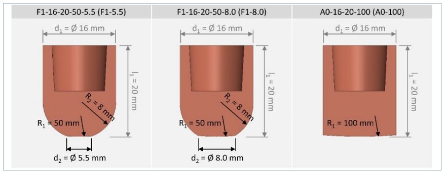
Methods for avoidance of LME also were investigated. Changing the electrode tip geometry to larger working plane diameters and elongating the hold time proved to eliminate LME cracks. In the experiments, a change of electrode tip geometry from a 5.5 mm to an 8.0 mm (Figure 4) enabled LME-free welds even when doubling the weld times above 600 ms. Using a flat-headed cap (with small edge radii or beveled), even the most extreme welding schedules (weld times greater than 1000 ms) did not produce cracks. The in-depth analysis revealed that larger electrode tip geometries clearly reduce the local plastic deformation around the indentation. This plastic strain reduction is particularly important, as longer weld times contribute to a higher liquid zinc exposure interval, leading to a higher potential for LME cracks.
Figure 4: Electrode Geometries Used in Study Experiments
It was also seen that as more energy flows into a spot weld, it becomes more critical to parameterize an appropriate hold time. Depending on the scenario, the selection of the correct hold time alone can make the difference between cracked and crack-free welds. Insufficient hold times allow liquid zinc to remain on the steel surface and increased thermal stresses that form after the lift-off of the electrode caps. Elongated hold times reduce surface temperatures, minimizing surface stresses and thus LME potential.
Non-Destructive Testing: Laboratory and Production Capabilities
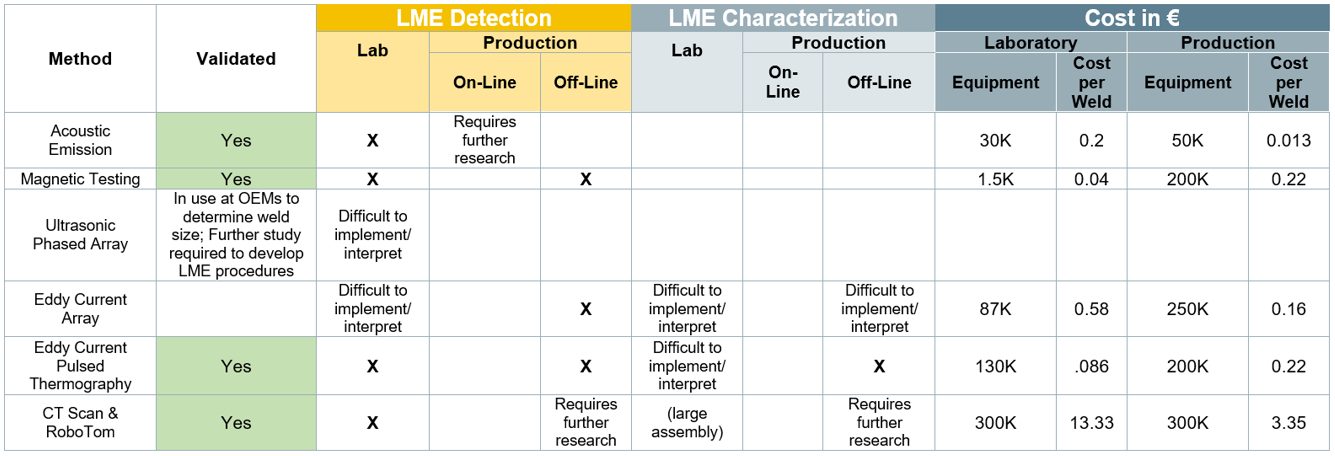
A third element of the study, and an aid in the control of LME, is the detection and characterization of LME cracks in resistance spot welds, either in laboratory or in production conditions. This work was done by the Institute of Soudure in close cooperation with LWF, IPK and WorldAutoSteel members’ and other manufacturing facilities. Ten different non-destructive techniques and systems were investigated. These techniques can be complementary, with various levels of costs, with some solutions more technically mature than others. Several techniques proved to be successful in crack detection. In order to aid the production source, techniques must not only detect but also characterize cracks to determine intensity and the effect on joint strength. Further work is required to achieve production-level characterization.
The study report provides detailed technical information concerning the experimental findings and performances of each technique/system and the possible application cost of each. Table 1 shows a summary of results:
Table 1: Summary of NDT: LME Detection and Characterization Methods
Preventing LME
Suitable measures should always be adapted to the specific use case. Generally, the most effective measures for LME prevention or mitigation are:
Avoidance of excessive heat input (e.g. excess welding time, current).
Avoidance of sharp edges on spot welding electrodes; instead use electrodes with larger working plane diameter, while not increasing nugget-size.
Employing extended hold times to allow for sufficient heat dissipation and lower surface temperatures.
Avoidance of improper welding equipment (e.g. misalignments of the welding gun, highly worn electrodes, insufficient electrode cooling)
In conclusion, a key finding of this study is that LME cracks only occurred in the study experiments when there were deviations from proper welding parameters and set-up. Ensuring these preventive measures are diligently adhered to will greatly reduce or eliminate LME from the manufacturing line. For an in-depth review of the study and its findings, you can download a copy of the full report at worldautosteel.org.
LME Study Authors
The LME study authors were supported by a committed team of WorldAutoSteel member companies’ Joining experts, who provided valuable guidance and feedback.
Related Articles: More on this study in previous AHSS Insights blogs: