Conventional HSS, Steel Grades
ULC, IF, VD-IF, and EDDS are interchangeable terms that describe the most formable (high n-value) and lowest strength grade of steel. Adding phosphorus, manganese, and/or silicon to these grades increases the strength due to solid solution strengthening, precipitation of carbides and/or nitrides, and grain refinement.
For most alloys, steelmaking practices attempt to reduce phosphorus to very low levels, since increased phosphorus content is sometimes associated with an increased risk of embrittlement. However, in the ladle metallurgy station after steelmaking, small controlled amounts of phosphorus are added back to the melt when certain grades are produced, leading to the term “rephosphorized.” Phosphorus is a potent solid solution strengthening element, where only small additions result in large increases in yield and tensile strength.
When phosphorus or other solid solution strengthening elements are used to increase the strength of interstitial-free steels, IF-HS (Interstitial-Free High Strength) steel is produced. Using phosphorus leads to the term IF-Rephosphorized steel, or IF-Rephos.
These alloys have composition controlled to improve r-value. In some products, small amounts of boron are added to counteract the embrittlement effects brought on by the phosphorus.
These higher strength IF-HS grades are widely used for both structural and closure applications. Work hardening from forming increases panel strength, which is why they may be described as dent resistant steels. However, this alloying approach is not capable of producing a bake hardenable grade.
Compared bake hardenable steels, carbon-manganese steels, and HSLA steels at similar strength levels, IF-HS grades are more formable, resulting from the ultra-low carbon chemistry and interstitial-free microstructure.
Some of the specifications describing uncoated cold rolled interstitial-free high strength (IF-HS) steel are included below, with the grades typically listed in order of increasing minimum yield strength and ductility. Different specifications may exist. Many automakers have proprietary specifications which encompass their requirements. Note that EN and VDA terminology is based on minimum yield strength, while JFS standard is based on minimum tensile strength.
- EN10268, with the terms HC180Y, HC220Y, and HC260Y D-17
- VDA239-100, with the terms CR160IF, CR180IF, CR210IF, and CR240IF V-3
- JFS A2001, with the terms JSC340P, JSC370P, JSC390P, and JSC440P J-23
![Crash Management]()
Crash Management, structural performance
In addition to enhanced formability, Advanced High-Strength Steels (AHSS) provide crash energy management benefits over their conventional High-Strength Steel (HSS) counterparts at similar strength levels. Higher levels of work hardening and bake hardening at a given strength level contribute to this improvement in crash performance.
The energy required for plastically deforming a material (force times distance) has the same units as the area under the true stress-true strain curve. This applies to all types of plastic deformation – from that which occurs during tensile testing, stamping, and crash. The major difference between these is the speed at which the deformation takes place.
As an example, consider the press energy requirements of two grades by comparing the respective areas under their true stress – true strain curves. The shape and magnitude of these curves are a function of the yield strength and work hardening behavior as characterized by the n-value when tested at conventional tensile testing speeds. At the same yield strength, a grade with higher n-value will require greater press energy capability, as highlighted in Figure 1 which compares HSLA 350/450 and DP 350/600. For these specific tensile test results, there is approximately 30% greater area under the DP curve compared with the HSLA curve, suggesting that forming the DP grade requires 30% more energy than required to form a part using the HSLA grade.

Figure 1: True stress-strain curves for two materials with equal yield strength.T-3
The high degree of work hardening exhibited by DP and TRIP steels results in higher ultimate tensile strength than that exhibited by conventional HSS of similar yield strength. This provides for a larger area under the true stress-strain curve. Similarly, when panels are formed from these grades, the work hardening during forming leads to higher in-panel strength than panels from HSS of comparable yield strength, further increasing the area under the stress-strain curve, ultimately resulting in greater absorption of crash energy.
Finally, the high work-hardening rate better distributes strain during crash deformation, providing for more stable, predictable axial crush that is crucial for maximizing energy absorption during a front or rear crash event.
Many AHSS are bake hardenable. The relatively large BH effect also increases the energy absorption capacity of these grades by further increasing the area under the stress-strain curve. The BH effect adds to the work hardening imparted by the forming operation. Conventional HSS do not exhibit a strong BH effect and therefore do not benefit from this strengthening mechanism.
Figure 2 illustrates the difference in energy absorption between DP and TRIP steels as a function of their yield strength determined at quasi-static tensile testing speeds.

Figure 2: Absorbed energy for square tube as function of quasi-static yield strength.T-2
Figure 3 shows calculated absorbed energy plotted against total elongation for a square tube component. The absorbed energy remains constant for the DP and TRIP steels but the increase in total elongation allows for formation into complex shapes.

Figure 3: Calculated absorbed energy for a square tube as a function of total elongation.T-2
For certain parts, conventional steels may have sufficient formability for stamping, yet lack the required ductility for the desired crash failure mode and will split prematurely rather than collapsing in a controlled manner. AHSS grades improve energy absorption by restoring a stable crush mode, permitting more material to absorb the crash energy. The increased ductility of AHSS grades permit the use of higher strength steels with greater energy absorbing capacity in complex geometries that could not otherwise be formed from conventional HSS alloys.
Stable and predictable deformation during a crash event is key to optimizing the steel alloy selection. The ideal profile is a uniform folding pattern showing progressive buckling with no cracks (Figure 4).

Figure 4: Deformation after axial crushing.A-49
Achieving crack-free folds is related to the local formability of the chosen alloy. Insufficient bendability can lead to early failure (Figure 5). Research to determine proper simulation inputs with physical testing for verification.

Figure 5: Three-point bend testing of two DP980 products having different folding and cracking behavior resulting from different microstructures and alloying approaches.B-12
High Strain Rate Property Test Methods
for Steel and Competing Materials
Tensile testing occurs at speeds that are 1000x slower than typical automotive stamping rates. Furthermore, automotive stamping is done at speeds that are 100x to 1000x slower than crash events. Stress-strain responses change with test speed – sometimes quite dramatically.
The m-value is one parameter to characterize this effect, since it is a measure of strain rate sensitivity. Generally, steel has more favorable strain rate effect properties compared with aluminum, but this is also a function of alloy, test temperature, selected strain range, and test speed. L-20
These reasons form the background for the need to characterize the intermediate and high strain rate behavior of AHSS.
![Crash Management]()
Formability
topofpage
If all stampings looked like a tensile dogbone and all deformation was in uniaxial tension, then a tensile test would be sufficient to characterize the formability of that metal. Obviously, engineered stampings are much more complex. Although a tensile test characterizes one specific strain path, a Forming Limit Curve (FLC) is necessary to have a map of strains indicating the onset of critical through-thickness necking for different linear strain paths. The strains which make up the FLC represent the limit of useful deformation. Calculations of safety margins are based on the FLC (Figure 1).

Figure 1: General graphical form of the Forming Limit Curve.E-2
Picturing a blank covered with circles helps visualize strain paths. After forming, the circles turn into ellipses, with the dimensions related to the major and minor strains. This forms the basis for Circle Grid Strain Analysis.
Generating Forming Limit Curves from Equations
Pioneering work by Keeler, Brazier, Goodwin and others contributed to the initial understanding of the shape of the Forming Limit Curve, with the classic equation for the lowest point on the FLC (termed FLC0) based on sheet thickness and n-value. Dr. Stuart Keeler was the Technical Editor of these AHSS Guidelines through Version 6.0, released in 2017.
 |
Equation 1 |
These studies generated the left hand side of the FLC as a line of constant thinning in true strain space, while the right hand side has a slope of +0.6, at least through minor (engineering) strains of 20%.
Evidence accumulated over many decades show that this approach to defining the Forming Limit Curve is sufficient for many applications of mild steels, conventional high strength steels, and some lower strength AHSS grades like CR340Y/590T-DP. However, this basic method is insufficient when it comes to creating the Forming Limit Curves for most AHSS grades and every other sheet metal alloy. Grades with significant amounts of retained austenite experience significant deviations from these simple estimates.H-23, S-61 In these cases, the FLC must be experimentally determined.
Additional studies found correlation with other properties including total elongation, tensile strength, and r-valueR-8, P-19, G-23, A-45, A-46, H-23 with some of these attempting to define the FLC by equations.
Experimental Determination of Forming Limit Curves
ASTM A-47 and ISO I-16 have published standards covering the creation of FLCs. Even within these standards, there are many nuances left for interpretation, primarily related to the precise definition of when a neck occurs and the associated limiting strains.
There are two steps in creating FLCs: Forming the samples and measuring the strains.
Forming sheet specimens of different widths uses either a hemispherical dome (Nakajima or Nakazima method N-14) or a flat-bottom punch (Marciniak method M-22) to generate different strain paths from which critical strains are determined. The two methods are not identical due to the different strain paths generated from the punch shape. These differences may not be significant for many lower strength and conventional High-Strength Steels, but may deviate from each other at higher strengths or with advanced microstructures. Figure 2 highlights samples formed with the Nakajima method.
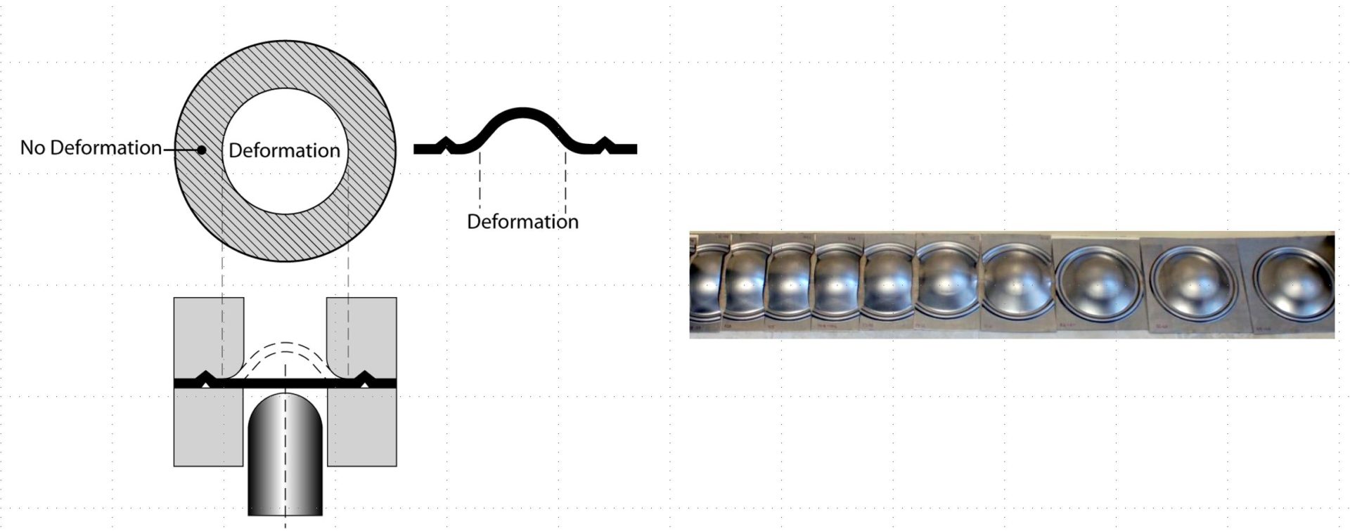
Figure 2: Forming limit curves can be created by deforming multiple samples of different widths. Narrow strips on the left allow metal to flow in from the unconstrained edges, creating a draw deformation mode leading to strains that plot on the left side of the FLC. Fully constrained samples, shown on the rightE-2, create a stretch deformation mode leading to strains that plot on the right side of the FLC.
Generally, strains are measured using one of two methods. The first approach involves covering the initially flat test samples with a grid pattern of circles, squares, or dots of known diameter and spacing to measure the strains associated with deformation. An alternate approach is based on Digital Image Correlation (DIC), where a camera tracks the movement of a random speckle pattern applied prior to forming.W-26, H-22, M-21 DIC methods are directly suited for use with stress-based FLCs.
Differences between Forming Limit Curves
and Forming Limit Diagrams
Often, the terms Forming Limit Curve (FLC) and Forming Limit Diagram (FLD) are used interchangeably. Perhaps a better way of categorizing is to define the components and what they encompass. This is somewhat of a simplification, since detailed interactions are known to occur.
- The Forming Limit Curve is a material parameter reflecting of the limiting strains resulting in necking failure as a function of strain path. It is a function of the metal grade, thickness, and sheet surface conditions, as well as the methods used during its creation (hemispherical/flat punch, test speed, temperature). It is applicable to any part shape.
- Deforming a flat sheet into an engineered stamping results in a formed surface with strains as a function of the forming conditions like local radii, lubrication, friction, and of course part geometry. These strains are essentially independent of the chosen metal grade and thickness. Plotting these strains allows for a relative assessment of which strains are higher than others, but no judgment can be made on “how high is too high?”
- The Forming Limit Diagram is a combination of the Forming Limit Curve (a material property) and the strains (reflecting part geometry and forming conditions). The FLD provides guidance on which areas of the formed part requires additional attention to achieve robust stamping conditions. Creating a subsequent FLD may be warranted when conditions change, since changes to the sheet metal properties (FLC) and the forming conditions (radii, lubrication, beads, blank size) will change the FLD, potentially affecting the conclusions.
Key Points
-
- Conventional Forming Limit Curves characterize necking failure only. Fractures at cut edges and tight bends may occur at strains lower than that suggested by the Forming Limit Curve.
- Differences in determination and interpretation of FLCs exist in different regions of the world.
- This system of FLCs commonly used for low strength and conventional HSLA is generally applicable to experimental FLCs obtained for DP steels for global formability.
- The left side of the FLC (negative minor strains) is in good agreement with experimental data for DP and TRIP steels. The left side depicts a constant thinning strain as a forming limit.
- Determination of FLCs for TRIP, MS, TWIP, and other special steels typically requires an experimental approach, since conventional simple equations do not accurately reflect the forming limits for these advanced microstructures.
Back to the Top
Formability
A Forming Limit Curve (FLC) is a map of strains indicating the onset of critical through-thickness necking for different linear strain paths. The FLC is dependent on the metal grade and the specific methods used in its creation. When paired with the strains generated during forming of an engineered part, the associated Forming Limit Diagram (FLD) provides guidance on which areas of the part might be prone to necking failures during production stamping conditions that replicate those used in the analysis.
Several methods are available to measure the strains on formed parts. The earliest method is known as Circle Grid Strain Analysis (CGSA), with Dr. Stuart Keeler as its primary evangelist for nearly 50 years. Dr. Keeler was the Technical Editor of these AHSS Guidelines through Version 6.0, released in 2017.
As the name suggests, a flat blank is covered with a grid of circles of precisely known diameter, typically applied by electrochemical etching. Forming turns the circles into ellipses, with the dimensions related to the major and minor strains. Conventional measurement occurs after forming, and involves a calibrated Mylar™ strip marked with gradations indicating the expansion or contraction relative to the initial circle diameter. Typically, these are viewed through magnifiers, making it easier to discern the critical dimensional differences. Techniques and caveats are highlighted in Citations S-59 and S-60.
Instead of circles, most camera-based measurement techniques for analysis after forming use a regular grid pattern of squares or dots. Forming turns the squares into rectangles, and the camera/computer measures the expansion or contraction of the nodes at the corners of the squares to determine the strains. Similarly, forming changes the regular dot pattern, allowing for calculation of the strains.
These approaches determine only the strains after forming, and are constrained to assume linear strain paths. An alternate approach based on Digital Image Correlation (DIC), where a camera tracks the movement of a random speckle pattern applied prior to forming,W-26, H-22, M-21 follows the strain evolution which occurs during forming and is not affected by non-linear strain paths.
Although DIC strain analysis is more accurate and informative, it is a higher-cost approach best suited for laboratory environments. Circle-grid, square-grid, and dot-grid strain analysis are all lower cost options and readily applied on the shop floor. Each of these in-plant techniques have different merits and challenges, including ease of use, accuracy, and cost.
Citations
Citation:
T-43. Courtesy of Türk Otomobil Fabrikası A.Ş. (Tofas).