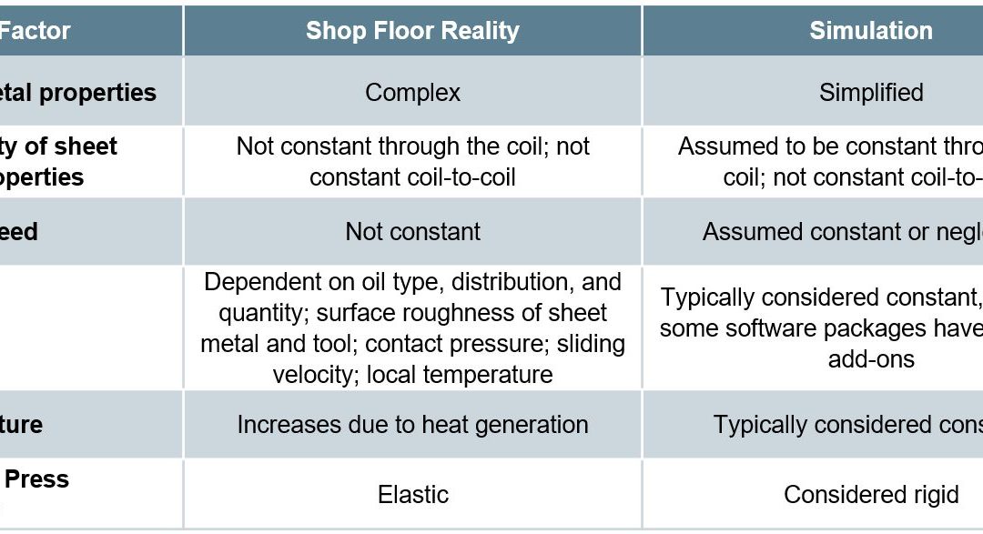
Simulation
Predicting metal flow and failure is the essence of sheet metal forming simulation. Characterizing the stress-strain response to metal flow requires a detailed understanding of when the sheet metal first starts to permanently deform (known as the yield criteria), how the metal strengthens with deformation (the hardening law), and the failure criteria (for example, the forming limit curve). Complicating matters is that each of these responses changes as three-dimensional metal flow occurs, and are functions of temperature and forming speed.
The ability to simulate these features reliably and accurately requires mathematical constitutive laws that are appropriate for the material and forming environments encountered. Advanced models typically improve prediction accuracy, at the cost of additional numerical computational time and the cost of experimental testing to determine the material constants. Minimizing these costs requires compromises, with some of these indicated in Table I created based on Citations B-16 and R-28.
Table I: Deviations from reality made to reduce simulation costs. Based on Citations B-16 and R-28.
Yield Criteria
The yield criteria (also known as the yield surface or yield loci) defines the conditions representing the transition from elastic to plastic deformation. Assuming uniform metal properties in all directions allows for the use of isotropic yield functions like von Mises or Tresca. A more realistic approach considers anisotropic metal flow behavior, requiring the use of more complex yield functions like those associated with Hill, Barlat, Banabic, or Vegter.
No one yield function is best suited to characterize all metals. Some yield functions have many required inputs. For example, “Barlat 2004-18p” has 18 separate parameters leading to improved modeling accuracy – but only when inserting the correct values. Using generic textbook values is easier, but negates the value of the chosen model. However, determining these variables typically is costly and time-consuming, and requires the use of specialized test equipment.
Hardening Curve
Metals get stronger as they deform, which leads to the term work hardening. The flow stress at any given amount of plastic strain combines the yield strength and the strengthening from work hardening. In its simplest form, the stress-strain curve from a uniaxial tensile test shows the work hardening of the chosen sheet metal. This approach ignores many of the realities occurring during forming of engineered parts, including bi-directional deformation.
Among the simpler descriptions of flow stress are those from Hollomon, Swift, and Ludvik. More complex hardening laws are associated with Voce and Hockett-Sherby.
The strain path followed by the sheet metal influences the hardening. Approaches taken in the Yoshida-Uemori (YU) and the Homogeneous Anisotropic Hardening (HAH) models extend these hardening laws to account for Bauschinger Effect deformations (the bending-unbending associated with travel over beads, radii, and draw walls).
As with the yield criteria, accuracy improves when accounting for three-dimensional metal flow, temperature, and forming speed, and using experimentally determined input parameters for the metal in question rather than generic textbook values.
Failure Conditions
Defining the failure conditions is the other significant challenge in metal forming simulation. Conventional Forming Limit Curves describe necking failure under certain forming modes, and are easier to understand and apply than alternatives. Complexity and accuracy increase when accounting for non-linear strain paths using stress-based Forming Limit Curves. Necking failure is not the only type of failure mode encountered. Conventional FLCs cannot predict fracture on tight radii and cut edges, nor can they account for dimensional issues like springback. For these, failure criteria definitions which are more mathematically complex are appropriate.
Constitutive Laws and Their Influence
on Forming Simulation Accuracy
Many simulation packages allow for an easy selection of constitutive laws, typically through a drop-down menu listing all the built-in choices. This ease potentially translates into applying inappropriate selections unless the simulation analyst has a fundamental understanding of the options, the inputs, and the data generation procedures.
Some examples:
- The “Keeler Equation” for the estimation of FLC0 has many decades of evidence in being sufficiently accurate when applied to mild steels and conventional high strength steels. The simple inputs of n-value and thickness make this approach particularly attractive. However, there is ample evidence that using this approach with most advanced high strength steels cannot yield a satisfactory representation of the Forming Limit Curve.
- Even in cases where it is appropriate to use the Keeler Equation, a key input is the n-value or the strain hardening exponent. This value is calculated as the slope of the (natural logarithm of the true stress):(natural logarithm of the true strain curve). The strain range over which this calculation is made influences the generated n-value, which in turn impacts the calculated value for FLC0.
- The strain history as measured by the strain path at each location greatly influences the Forming Limit. However, this concept has not gained widespread understanding and use by simulation analysts.
- A common method to experimentally determine flow curves combines tensile testing results through uniform elongation with higher strain data obtained from biaxial bulge testing. Figure 1 shows a flow curve obtained in this manner for a bake hardenable steel with 220 MPa minimum yield strength. Shown in Figure 2 is a comparison of the stress-strain response from multiple hardening laws associated with this data, all generated from the same fitting strain range between yield and tensile strength. Data diverges after uniform elongation, leading to vastly different predictions. Note that the differences between models change depending on the metal grade and the input data, so it is not possible to say that one hardening law will always be more accurate than others.

Figure 1: Flow curves for a bake hardenable steel generated by combining tensile testing with bulge testing.L-20

Figure 2: The chosen hardening law leads to vastly different predictions of stress-strain responses.L-20
- Analysts often treat Poisson’s Ratio and the Elastic Modulus as constants. It is well known that the Bauschinger Effect leads to changes in the Elastic Modulus, and therefore impacts springback. However, there are also significant effects in both Poisson’s Ratio (Figure 3) and the Elastic Modulus (Figure 4) as a function of orientation relative to the rolling direction. Complicating matters is that this effect changes based on the selected metal grade.

Figure 3: Poisson’s Ratio as a Function of Orientation for Several Grades (Drawing Steel, DP 590, DP 980, DP 1180, and MS 1700) D-11

Figure 4: Modulus of Elasticity as a Function of Orientation for Several Grades (Drawing Steel, DP 590, DP 980, DP 1180, and MS 1700) D-11
Complete material card development requires results from many tests, each attempting to replicate one or more aspects of metal flow and failure. Certain models require data from only some of these tests, and no one model typically is best for all metals and forming conditions. Tests described below include:
- Tensile testing [room temperature at slow strain rates to elevated temperature with accelerated strain rates]
- Biaxial bulge testing
- Biaxial tensile testing
- Shear testing
- V-bending testing
- Tension-compression testing with cyclic loading
- Friction
Tensile testing is the easiest and most widely available mechanical property evaluation required to generate useful data for metal forming simulation. However, a tensile test provides a complete characterization of material flow only when the engineered part looks like a dogbone and all deformation resulted from pulling the sample in tension from the ends. That is obviously not realistic. Getting tensile test results in more than just the rolling direction helps, but generating those still involves pulling the sample in tension. Three-dimensional metal flow occurs, and the stress-strain response of the sheet metal changes accordingly.
The uniaxial tensile test generates a draw deformation strain state since the edges are free to contract. A plane strain tensile test requires using a modified sample geometry with an increased width and decreased gauge length,
Forming all steels involves a thermal component, either resulting from friction and deformation during “room temperature” forming or the intentional addition of heat such as used in press hardening. In either case, modeling the response to temperature requires data from tests occurring at the temperature of interest, at appropriate forming speeds. Thermo-mechanical simulators like Gleeble™ generate such data.
Conventional tensile testing occurs at deformation rates of 0.001/sec. Most production stamping occurs at 10,000x that amount, or 10/sec. Crash events can be 2 orders of magnitude faster, at about 1000/sec. The stress-strain response varies by both testing speed and grade. Therefore, accurate simulation models require data from higher-speed tensile testing. Typically, generating high speed tensile data involves drop towers or Split Hopkinson Pressure Bars.
A pure uniaxial stress state exists in a tensile test only until reaching uniform elongation and the beginning of necking. Extrapolating uniaxial tensile data beyond uniform elongation risks introducing inaccuracies in metal flow simulations. Biaxial bulge testing generates the data for yield curve extrapolation beyond uniform elongation. This stretch-forming process deforms the sheet sample into a dome shape using hydraulic pressure, typically exerted by water-based fluids. Citation I-12 describes a standard test procedure for biaxial bulge testing.
A Marciniak test used to create Forming Limit Curves generates in-plane biaxial strains. Whereas FLC generation uses 100 mm diameter samples, larger samples allow for extraction of full-size tensile bars. Although this approach generates samples containing biaxial strains, the extracted samples are tested uniaxially in the conventional manner.
Biaxial tensile testing allows for the determination of the yield locus and the biaxial anisotropy coefficient, which describes the slope of the yield surface at the equi-biaxial stress state. This test uses cruciform-shaped test pieces with parallel slits cut into each arm. Citation I-13 describes a standard test procedure for biaxial tensile testing. The biaxial anisotropy coefficient can also be determined using the disk compression testing as described in Citation T-21.
Shear testing characterizes the sheet metal in a shear loading condition. There is no consensus on the specimen type or testing method. However, the chosen testing set-up should avoid necking, buckling, and any influence of friction.
V-bending tests determine the strain to fracture under specific loading conditions. Achieving plane strain or plane stress loading requires use of a test sample with features promoting the targeted strain state.
Tension-compression testing characterizes the Bauschinger Effect. Multiple cycles of tension-compression loading captures cyclic hardening behavior and elastic modulus decay, both of which improve the accuracy of springback predictions. Again, no standard procedure exists. The biggest challenge with this test is preventing buckling from occurring during in-plane compressive loading. Related to this is the need to compensate for the friction caused by the anti-buckling mechanism in the stress-strain curves .
Friction is obviously a key factor in how metal flows. However, there is no one simple value of friction that applies to all surfaces, lubricants, and tooling profiles. The coefficient of friction not only varies from point to point on each stamping but changes during the forming process. Determining the coefficient of friction experimentally is a function of the testing approach used. The method by which analysts incorporate friction into simulations influences the accuracy and applicability of the results of the generated model.
Studies are underway to reduce the costs and challenges of obtaining much of this data. It may be possible, for example, to use Digital Image Correlation (DIC) during a simple uniaxial tensile testing to quantify r-value at high strains, determine the material hardening behavior along with strain rate sensitivity, assess the degradation of Young’s Modulus during unloading, and use the detection of the onset of local neck to help account for non-linear strain path effects.S-110
Application of Advanced Testing to Failure Predictions
Global formability failures occur when the forming strains exceed the necking forming limit throughout the entire thickness of the sheet. Advanced steels are at risk of local formability failures where the forming strains exceed the fracture forming limit at any portion of the thickness of the sheet.
Fracture forming limit curves plot higher than the conventional necking forming limit curves on a graph showing major strain on the vertical axis and minor strain on the horizontal axis. In conventional steels the gap between the fracture FLC and necking FLC is relatively large, so the part failure is almost always necking. The forming strains are not high enough to reach the fracture FLC.
In contrast, AHSS grades are characterized by a smaller gap between the necking FLC and the fracture FLC. Depending on the forming history, part geometry (tight radii), and blank processing (cut edge quality), forming strains may exceed the fracture FLC at an edge or bend before exceeding the necking FLC through-thickness. In this scenario, the part will fracture without signs of localized necking.
A multi-year study funded by the American Iron and Steel Institute at the University of Waterloo Forming and Crash Lab describes a methodology used for forming and fracture characterization of advanced high strength steels, the details of which can be found in Citations B-11, W-20, B-12, B-13, R-5, N-13 and G-19.
This collection of studies, as well as work coming out of these studies, show that relatively few tests sufficiently characterize forming and fracture of AHSS grades. These studies considered two 3rd Gen Steels, one with 980MPa tensile strength and one with 1180MPa tensile.
- The yield surface as generated with the Barlat YLD2000-2d yield surface (Figure 5) comes from:
- Conventional tensile testing at 0, 22.5, 45, 67.5, and 90 degrees to the rolling direction, determining the yield strength and the r-value;
- Disc compression tests according to the procedure in Citation T-21 to determine the biaxial R-value, rb.

Figure 5: Tensile testing and disc compression testing generate the Barlat YLD2000-2d yield surface in two 3rd Generation AHSS Grades B-13
- Creating the hardening curve uses a procedure detailed in Citations R-5 and N-13, and involves only conventional tensile and shear testing using the procedure included in Citation P-15.

Figure 6: Test geometries for hardening curve generation. Left image: Tensile; Right image: Shear.N-13
- Characterizing formability involved generating a Forming Limit Curve using Marciniak data or process-corrected Nakazima data. (See our article on non-linear strain paths) and Citation N-13 for explanation of process corrections]. Either approach resulted in acceptable characterizations.
- Fracture characterization uses four plane stress tests: shear, conical hole expansion, V-bending, and a biaxial dome test. The result from these tests calibrate the fracture locus describing the stress states at fracture.
Back To Top
![Cutting, Blanking, Shearing & Trimming]()
Cutting, Cutting-Blanking-Shearing-Trimming
Advanced High-Strength Steels (AHSS) exhibit high degrees of work hardening, resulting in improved forming capabilities compared to conventional HSLA steels. However, the same high work hardening creates higher strength and hardness in sheared or punched edges, leading to reduced edge ductility. Microstructural features in some AHSS grades contribute to their sheared edge performance. While laser cutting results in less edge damage than mechanical cutting methods, the heat from laser cutting produces a localized hear treatment, changing the strength and hardness at the edge. Achieving the best formability for chosen processing path requires generating a consistent good quality edge from the cutting operation.
To avoid unexpected problems during a program launch, use production intent tooling as early in the development as possible. This may be a challenge since blanking dies are usually among the last set of tools completed. In the interim, many companies choose to use laser cut blanks. Tool, blank, and process development must account for the lower-ductility sheared edges in production blanks.
Edge Ductility Measurements
This article describes the impact of cutting and cut-edge quality on edge ductility. The primary tests which quantify edge ductility are Hole Expansion Testing, 2-D Edge Tension Testing, and Half Specimen Dome Testing. These links detail the testing procedures. The Hole Expansion Testing article has additional information pertaining to the effect of burr orientation and punch shape.
Cut Edge Quality
Any mechanical cutting operation such as blanking, piercing, shearing, slitting, or trimming reduces edge ductility. Each of these processes generate a zone of high work hardening and a reduced n-value. This work hardened zone can extend one-half metal thickness from the cut edge. This is one reason why edges fail at strains lower than that predicted by the forming limit curve for that particular grade (Note that FLCs were developed based on necking failure, and that edge cracking is a different failure mechanism).
DP and TRIP steels have islands of martensite located throughout the ferritic microstructure, including at the cut edges. These hard particles act as crack initiators and further reduce the allowable edge stretch. Metallurgical changes to the alloy minimize the hardness differences between the phases, resulting in improved edge ductility. Laser, EDM or water jet cutting approaches minimize work hardening at the edges and the associated n-value reduction, also leading to improved edge ductility.
Putting shear angles into cutting tools is a well-known approach to reduce cutting forces. Modifying the cutting tool leads to other benefits in terms of edge ductility. Researchers studied the effects of a beveled punch instead of the traditional flat bottom punch.S-9, S-50, S-52 In these studies, the optimized bevel angle was between 3 and 6 degrees, the shear direction was parallel the rolling direction of the coil with a die clearance of 17%. With the optimal cutting parameters, the hole expansion ratio increased by 60% when compared to conventional flat punching process. As expected, a reduction in the maximum shearing force occurred – by more than 50% in certain conditions. Dropping the shearing force helps reduce the snap through reverse tonnage, leading to longer tool and press life.
Multiple studies examine the trimmed edge quality based on various cutting conditions in mechanical shearing operations and other methods to produce a free edge such as milling and cutting using a laser or water jet. Edge quality varies based on parameters like cutting clearances, shear angles, and rake angles on mechanical shearing operations.
A typical mechanically sheared steel edge has 4 main zones – rollover, burnish, fracture, and burr, as shown in Figure 1.

Figure 1: Cross Section of a Punched Hole Showing the Shear Face Components and Shear Affected Zone.K-10
Parts stamped from conventional mild and HSLA steels have historically relied on burr height as the main measure of edge quality, where the typical practice targeted a burr height below 10% of metal thickness and slightly larger for thicker steel. Finding a burr exceeded this threshold usually led to sharpening or replacing the trim steels, or less likely, adjusting the clearances to minimize the burr.
Greater burr height is associated with additional cold working and creates stress risers that can lead to edge splitting. These splits, however, are global formability related failures where the steel thins significantly at and around the split, independent of the local formability edge fractures associated with AHSS. A real-world example is shown in Figure 2, which presents a conventional BH210 steel grade liftgate with an excessive burr in the blank that led to global formability edge splitting in the draw die. The left image in Figure 2 highlights the burr on the underside of the top blank, with the remainder of the lift below it. The areas next to the split in the right image of Figure 2 shows the characteristic thinning associated with global formability failures.
Figure 2: Excessive burr on the blank led to a global formability split on the formed liftgate. The root cause was determined to be dull trim steels resulting in excessive work hardening.U-6
Due to their progressively higher yield and tensile strengths, AHSS grades experience less rollover and smaller burrs. They tend to fracture with little rollover or burr. As such, detailed examination of the actual edge condition under various cutting conditions becomes more significant with AHSS as opposed characterizing edge quality by burr height alone. Examination of sheared edges produced under various trimming conditions, including microhardness testing to evaluate work hardening after cold working the sheared edge, provides insight on methods to improve cut edge formability. The ideal condition to combat local formability edge fractures for AHSS was to have a clearly defined burnish zone with a uniform transition to the fracture zone. The fracture zone should also be smooth with no voids, secondary shear or edge damage (Figure 3).

Figure 3: Ideal sheared edge with a distinct burnish zone and a smooth fracture zone (left) and a cross section of the same edge (right).U-6
If clearances are too small, secondary shear can occur and the potential for voids due to the multiphase microstructure increases, as indicated in Figure 4. Clearances that are too large create additional problems that include excessive burrs and voids. A nonuniform transition from the burnish zone to the fracture zone is also undesirable. These non-ideal conditions create propagation sites for edge fractures.

Figure 4: Sheared edge with the trim steel clearance too small (left) and a cross section of the same edge (right) showing a micro crack on the edge. Tight clearance leading to secondary shear increases likelihood of edge fracture.U-6
There are multiple causes for a poor sheared edge condition, including but not limited to:
- the die clearance being too large or too small,
- a cutting angle that is too small,
- worn, chipped, or damaged tooling,
- improperly ground or sharpened tooling,
- improper die material,
- improperly heat-treated die material,
- improper (or non-existent) coating on the tooling,
- misaligned die sections,
- worn wear plates, and
- out of level presses or slitting equipment.
The higher loads required to shear AHSS with increasingly higher tensile strength creates additional deflection of dies and processing equipment. This deflection may alter clearances measured under a static condition once the die, press, or slitting equipment is placed under load. As a large percentage of presses, levelers, straighteners, blankers, and slitting equipment were designed years ago, the significantly higher loads required to process today’s AHSS may exceed equipment beyond their design limits, dramatically altering their performance.
A rocker panel formed from DP980 provides a good example showing the influence of cut edge quality. A master coil was slit into several narrower coils (mults) before being shipped to the stamper. Only a few mults experienced edge fractures, which all occurred along the slit edge. Understanding that edge condition is critical with respect to multiphase AHSS, the edge condition of the “good” mults and the “bad” mults were examined under magnification. The slit edge from a problem-free lift (Figure 5) has a uniform burnish zone with a uniform transition to the smooth fracture zone. This is in contrast with Figure 6, from the slit edge from a different mult of the same coil in which every blank fractured at the slit edge during forming. This edge exhibits secondary shear as well as a thick burnish zone with a non-uniform transition from the burnish zone to the fracture zone.

Figure 5: Slit edges on a lift of blanks that successfully produced DP980 rocker panels. Note the uniform transition from the burnish zone to the fracture zone with a smooth fracture zone as well.U-6

Figure 6: Slit edges on a lift of blanks from the same master coil that experienced edge fractures during forming. Note the obvious secondary shear as well as the thicker, nonuniform transition from the burnish to the fracture zone.U-6
Cutting Clearances: Burr Height and Tool Wear
Cutting and punching clearances should be increased with increasing sheet material strength. The clearances range from about 6% of the sheet material thickness for mild steel up to 16% or even higher as the sheet metal tensile strength exceeds 1400 MPa.
A study C-2 compared the tool wear and burr height formation associated with punching mild steel and several AHSS grades. In addition to 1.0 mm mild steel (140 MPa yield strength, 270 MPa tensile strength, 38% A80 elongation), AHSS grades tested were 1.0 mm samples of DP 350Y600T (A80=20%), DP 500Y800T (A80=8%), and MS 1150Y1400T (A80 = 3%). Tests of mild steel used a 6% clearance and W.Nr. 1.2363 / AISI A2 tool steel hardened to 61 HRC. The AHSS tests used engineered tool steels made from powder metallurgy hardened to 60-62 HRC. The DP 350/600 tests were run with a TiC CVD coating, and a 6% clearance. Tool clearances were 10% for the MS 1150Y1400T grade and 14% for DP 500Y800T.
In the Tool Wear comparison, the cross-section of the worn punch was measured after 200,000 hits. Punches used with mild steel lost about 2000 μm2 after 200,000 hits, and is shown in Figure 7 normalized to 1. The relative tool wear of the other AHSS grades are also shown, indicating that using surface treated high quality tool steels results in the same level of wear associated with mild steels punched with conventional tools.

Figure 7: Tool wear associated with punching up to DP 500Y800T using surface treated high quality tool steels is comparable to mild steel punched with conventional tools.C-2
Figure 8 shows the burr height test results, which compared burr height from tests using mild steel punched with conventional tool steel and two AHSS grades (DP 500Y800T and MS 1150Y1400T) punched with a PM tool steel. The measured burr height from all AHSS and clearance combinations evaluated were sufficiently similar that they are shown as a single curve.

Figure 8: Burr height comparison for mild steel and two AHSS grades as a function of the number of hits. Results for DP 500Y800T and Mart 1150Y1400T are identical and shown as the AHSS curve.C-2
Testing of mild steel resulted in the expected performance where burr height increases continuously with tool wear and clearance, making burr height a reasonable indicator of when to sharpen punching or cutting tools. However, for the AHSS grades studied, burr height did not increase with more hits. It is possible that the relatively lower ductility AHSS grades are not capable of reaching greater burr height due to fracturing, where the more formable mild steel continues to generate ever-increasing burr height with more hits and increasing tool wear.
Punching AHSS grades may require a higher-grade tool steel, possibly with a surface treatment, to avoid tool wear, but tool regrinding because of burrs may be less of a problem. With AHSS, engineered tool steels may provide longer intervals between sharpening, but increasing burr height alone should not be the only criterion to initiate sharpening: cut edge quality as shown in the above figures appears to be a better indicator. Note that regrinding a surface treated tool steel removes the surface treatment. Be sure to re-treat the tool to achieve targeted performance.
Cutting Clearances: General Recommendations
Depending on the source, the recommended die clearance when shearing mild steels is 5% to 10% of metal thickness. For punched holes, these represent per-side values. Although this may have been satisfactory for mild steels, the clearance should increase as the tensile strength of the sheet metal increases.
The choice of clearance impacts other aspects of the cutting process. Small cutting clearances require improved press and die alignment, greater punching forces, and cause greater punch wear from abrasion. As clearance increases, tool wear decreases, but rollover on the cut edge face increases, which in the extreme may lead to a tensile fracture in the rollover zone (Figure 9). Also, a large die clearance when punching high strength materials with a small difference in yield and tensile strength (like martensitic grades) may generate high bending stresses on the punch edge, which increases the risk of chipping.

Figure 9: Large rollover may lead to tensile fracture in the rollover zone.
Figure 10 compares cut edge appearance after punching a martensitic steel with 1400 MPa tensile strength using either 6% or 14% clearance. The larger clearance is associated with greater rollover, but a cleaner cut face.

Figure 10: Cut edge appearance after punching CR 1400T-MS with 6% (left) and 14% (right) die clearance. The bottom images show the edge appearance for the full sheet thickness, Note using 6% clearance resulted in minimal rollover, but uneven burnish and fracture surfaces. In contrast, 14% clearance led to noticeable rollover, but a clean burnish and fracture surface.T-20
A comparison of the edges of a 2 mm thick complex phase steel with 700 MPa minimum tensile strength produced under different cutting conditions is presented in Figure 11. The left image suggests that either the cutting clearance and/or the shearing angle was too large. The right image shows an optimal edge likely to result in good edge ductility.

Figure 11: Cut edge appearance of 2 mm HR 700Y-MC, a complex phase steel. The edge on the right is more likely to result in good edge ductility.T-20
The recommended clearance is a function of the sheet grade, thickness, and tensile strength. Figures 12 to 15 represent general recommendations from several sources.

Figure 12: Recommended Clearance as a Function of Grade and Sheet Thickness.T-23

Figure 13: Recommended Cutting Clearance for Punching.D-15

Figure 14: Recommended die clearance for blanking/punching advanced high strength steel.T-20

Figure 15: Multiply the clearance on the left with the scaling factor in the right to reach the recommended die clearance.D-16
Figure 16 highlights the effect of cutting clearance on CP1200, and reinforces that the historical rule-of-thumb guidance of 10% clearance does not apply for all grades. In this studyU-3, increasing the clearance from 10% to 15% led to a significant improvement in hole expansion. The HER resulting from a 20% clearance was substantially better than that from a 10% clearance, but not as good as achieved with a 15% clearance. These differences will not be captured when testing only to the requirements of ISO 16630, which specifies the use of 12% clearance.

Figure 16: Effect of hole punching clearance on hole expansion of Complex Phase steel grade CP1200.U-3
Cutting speed influences the cut edge quality, so it also influences the optimal clearance for a given grade. In a study published in 2020G-49, higher speeds resulted in better sheared edge ductility for all parameters evaluated, with those edges having minimal rollover height, smoother sheared surface and negligible burr. Two grades were evaluated: a dual phase steel with 780MPa minimum tensile strength and a 3rd Generation steel with 980 MPa minimum tensile strength.
Metallurgical characteristics of the sheet steel grade also affects hole expansion capabilities. Figure 17 compares the HER of DP780 from six global suppliers. Of course, the machined edge shows the highest HER due to the minimally work-hardened edge. Holes formed with 13% clearance produced greater hole expansion ratios than those formed with 20% clearance, but the magnitude of the improvement was not consistent between the different suppliers.K-56

Figure 17: Cutting clearance affects hole expansion performance in DP780 from six global suppliers.K-56
Punch Face Design
Practitioners in the field typically do not cut perpendicular to the sheet surface – angled punches and blades are known to reduce cutting forces. For example, long shear blades might have a 2 to 3 degree angle on them to minimize peak tonnages. There are additional benefits to altering the punch profile and impacting angle.
Snap-though or reverse tonnage results in stresses which may damage tooling, dies, and presses. Tools may crack from fatigue. Perhaps counter to conventional thinking, use of a coated punch increases blanking and punching forces. The coating leads to lower friction between the punch and the sheet surface, which makes crack initiation more difficult without using higher forces.
Unlike a coated tool, a chamfered punch surface reduces blanking and punching forces. Figure 18 compares the forces to punch a 5 mm diameter hole in 1 mm thick MS-1400T using different punch shapes. A chamfered punch was the most effective in reducing both the punching force requirements and the snap-through tonnage (the shock waves and negative tonnage readings in Figure 18). The chamfer should be large enough to initiate the cut before the entire punch face is in contact with the sheet surface. A larger chamfer increases the risk of plastic deformation of the punch tip.T-20

Figure 18: A chamfered punch reduces peak loads and snap-through tonnage.K-15
A different study P-16 showed more dramatic benefits. Use of a rooftop punch resulted in up to an 80% reduction in punching force requirements compared with a flat punch, with a significant reduction in snap-through tonnage. Cutting clearance had only minimal effect on the results. (Figure 19)

Figure 19: A rooftop-shaped punch leads to dramatic reductions in punch load requirements and snap-through tonnage.P-16
Use of a beveled punch (Figure 20) provides similar benefits. A study S-52 comparing DP 500/780 and DP 550/980 showed a reduction in the maximum piercing force of more than 50% with the use of a beveling angle between 3 and 6 degrees. The shearing force depends also upon the die clearance during punching, with the optimum performance seen with 17% die clearance. The optimal punching condition results in more than 60% improvement in the hole expansion ratio when compared to conventional flat head punching process. The optimal bevel cut edge in Figure 21 shows a uniform burnish zone with a uniform transition to the smooth fracture zone – the known conditions to produce a high-ductility edge.

Figure 20: Schematic showing a beveled punch.S-52

Figure 21: A bevel cut edge showing uniform burnish zone with a uniform transition to the smooth fracture zone.S-52
Effect of Edge Preparation Method on Ductility
A flat trim condition where the upper blade and lower blade motions are parallel and there is no shear rake angle is known to produce a trimmed edge with limited edge stretchability (Figure 22, left image). In addition to split parts, tooling damage and unexpected down time results. Metal stampers have known that shearing with a rake angle Figure 22, right image) will reduce cutting forces compared with using a flat cut. With advanced high strength steels, there is an accompanying reduction in forming energy requirements of up to 20% depending on the conditions, which represents a tremendous drop in snap-through or reverse tonnage. Figure 22 visually describes the upper and lower blade rake angles and the shear rake angle.
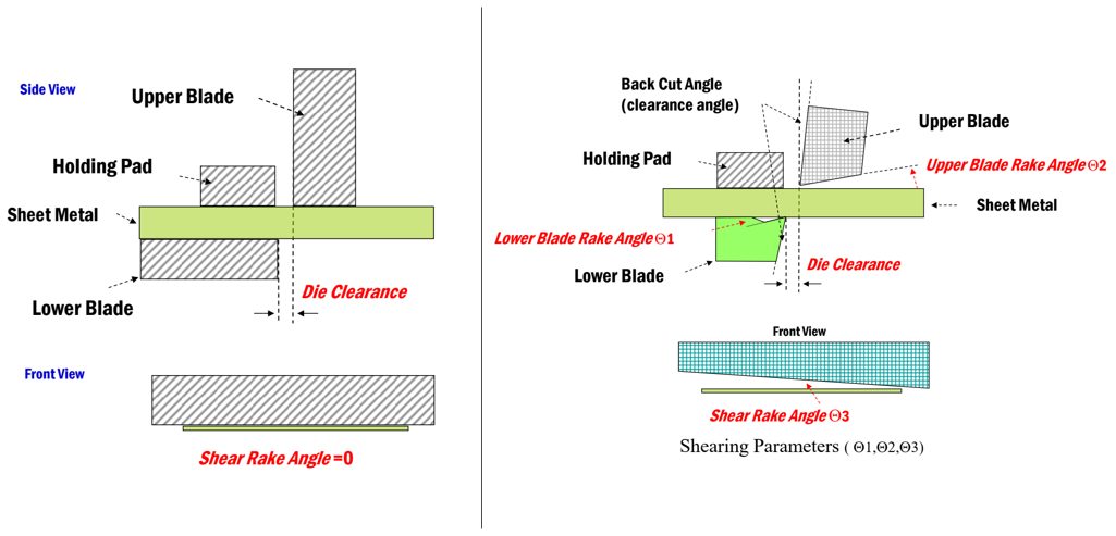
Figure 22: Flat trim (left) and shear trim (right) conditions showing rake angle definitions.S-53
Researchers have also found that it is possible to increase sheared edge ductility with optimized rake angles. Citation S-53 used 2-D Edge Tension Testing and the Half-Specimen Dome Test to qualify the effects of these rake angles, and determine the optimum settings. After preparing the trimmed edge with the targeted conditions, the samples were pulled in a tensile test or deformed using a hemispherical punch. The effect of the trimming conditions was seen in the measured elongation values and the strain at failure, respectively. The results are summarized in Figures 23-25. Some of the tests also evaluated milled, laser trimmed, and water jet cut samples. Shear Trim 1, 2, and 3 refer to the shear trim angle in degrees. The optimized shear condition also includes a 6-degree rake angle on both the upper and lower blades, as defined in Figure 22.
Conclusions from this study include:
- Mechanically shearing the edge cold works the steel and reduces the work hardening exponent (n-value), leading to less edge stretchability.
- Samples prepared with processes that avoided cold working the edges, like laser or water jet cutting outperformed mechanically sheared edges.
- Optimizing the trim shear conditions or polishing a flat trimmed edge approaches what can be achieved with laser trimming and water jet cutting.
- Shearing parameters such as clearance, shear angle and rake angle also play a large part in improving edge stretch.

Figure 23: Effect of edge preparation on stretchability as determined using a tensile test for DP 350Y600T (left) and DP 550Y980T (right).S-53

Figure 24: Effect of edge preparation on stretchability as determined using a dome test for DP 350Y600T (left) and DP 550Y980T (right).S-53

Figure 25: Optimizing the trim shear conditions or polishing a flat trimmed edge approaches what is achievable with laser trimming and water jet cutting. Data from dome testing of DP 350Y/600T.S-53
The optimal edge will have no mechanical damage and no microstructural changes as you go further from the edge. Any process that changes the edge quality from the bulk material can influence performance. This includes the mechanical damage from shearing operations, which cold works the edge leading to a reduction in ductility. Laser cutting also changes the edge microstructure, since the associated heat input is sufficient to alter the engineered balance of phases which give AHSS grades their unique properties. However, the heat from laser cutting is sometimes advantageous, such as in the creation of locally softened zones to improve cut edge ductility in some applications of press hardening steels.
The effects of edge preparation on the shear affected zone is presented in Figure 26. A flatter profile of the Vickers microhardness reading measured from the as-produced edge into the material indicates the least work-hardening and mechanical damage resulting from the edge preparation method, and therefore should result in the greatest edge ductility. This is certainly the case for water jet cutting, where a flat hardness profile in Figure 26 correlates with the highest ductility measurements in Figures 22 to 25. Unfortunately, water jet cutting is not always practical, and introduces the risk of rust forming at the newly cut edge.
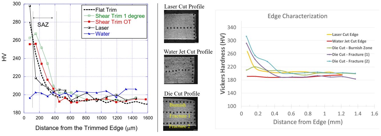
Figure 26: Microhardness profile starting at cut edge generated using different methods. Left image is from Citation S-53, and right image is from C-13.
Two-stage piercing is another method to reduce edge strain hardening effects. Here, a conventional piercing operation is followed by a shaving operation which removes the work-hardened material created in the first step, as illustrated in Figure 27.P-17 A related studyF-10 evaluated this method with a 4 mm thick complex phase steel with 800 MPa tensile strength. Using the configuration documented in this reference, single-stage shearing resulted in a hole expansion ratio of only 5%, where the addition of the shaving operation improved the hole expansion ratio to 40%.

Figure 27: Two-stage piercing improves cut edge ductility. Image adapted from Citation P-17.
Figure 28 highlights the benefits of two-stage pre-piercing for specific grades, showing a 2x to 4x improvement in hole expansion ratio for the grades presented.

Figure 28: Pre-piercing improves the hole expansion ratio of AHSS Grades.S-10
Key Points
- Clearances for punching, blanking, and shearing should increase as the strength of the material increases, but only up to a point. At the highest strengths, reducing clearance improves tool chipping risk.
- Lower punch/die clearances lead to accelerated tool wear. Higher punch/die clearances generate more rollover/burr.
- ISO 16630, the global specification for hole expansion testing, specifies the use of 12% punch-to-die clearance. Optimized clearance varies by grade, so additional testing may prove insightful.
- Recommended clearance as a percentage of sheet thickness increases with thickness, even at the same strength level.
- Burr height increases with tool wear and increasing die clearances for shearing mild steel, but AHSS tends to maintain a constant burr height. This means extended intervals between tool sharpening may be possible with AHSS parts, providing edge quality and edge performance remain acceptable.
- Edge preparation methods like milling, laser trimming, and water-jet cutting minimize cold working at the edges, resulting in the greatest edge ductility,
- Laser cut blanks used during early tool tryout may not represent normal blanking, shearing, and punching quality, resulting in edge ductility that will not occur in production. Using production-intent tooling as early as possible in the development stage minimizes this risk.
- Shear or bevel on punches and trim steel reduces punch forces, minimizes snap-through reverse tonnage, and improves edge ductility.
- Mild steel punched with conventional tools and AHSS grades punched with surface treated engineered PM tool steels experience comparable wear.
- Maintenance of key process variables, such as clearance and tool condition, is critical to achieving long-term edge stretchability.
- The optimal edge appearance shows a uniform burnish zone with a uniform transition to a smooth fracture zone.
Back To Top
![Cutting, Blanking, Shearing & Trimming]()
1stGen AHSS, AHSS, Steel Grades
Complex Phase (CP) steels combine high strength with relatively high ductility. The microstructure of CP steels contains small amounts of martensite, retained austenite and pearlite within a ferrite/bainite matrix. A thermal cycle that retards recrystallization and promotes Titanium (Ti), Vanadium (V), or Niobium (Nb) carbo-nitrides precipitation results in extreme grain refinement. Minimizing retained austenite helps improve local formability, since forming steels with retained austenite induces the TRIP effect producing hard martensite.F-11
The balance of phases, and therefore the properties, results from the thermal cycle, which itself is a function of whether the product is hot rolled, cold rolled, or produced using a hot dip process. Citation P-18 indicates that galvannealed CP steels are characterized by low yield value and high ductility, whereas cold rolled CP steels are characterized by high yield value and good bendability. Typically these approaches require different melt chemistry, potentially resulting in different welding behavior.
CP steel microstructure is shown schematically in Figure 1, with the grain structure for hot rolled CP 800/1000 shown in Figure 2. The engineering stress-strain curves for mild steel, HSLA steel, and CP 1000/1200 steel are compared in Figure 3.

Figure 1: Schematic of a complex phase steel microstructure showing martensite and retained austenite in a ferrite-bainite matrix.

Figure 2: Micrograph of complex phase steel, HR800Y980T-CP.C-14

Figure 3: A comparison of stress strain curves for mild steel, HSLA 350/450, and CP 1000/1200.
DP and TRIP steels do not rely on precipitation hardening for strengthening, and as a result, the ferrite in these steels is relatively soft and ductile. In CP steels, carbo-nitride precipitation increases the ferrite strength. For this reason, CP steels show significantly higher yield strengths than DP steels at equal tensile strengths of 800 MPa and greater. Engineering and true stress-strain curves for CP steel grades are shown in Figure 4.
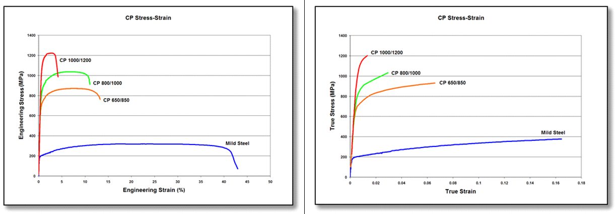
Figure 4: Engineering stress-strain (left graphic) and true stress-strain (right graphic) curves for a series of CP steel grades. Sheet thickness: CP650/850 = 1.5mm, CP 800/1000 = 0.8mm, CP 1000/1200 = 1.0mm, and Mild Steel = approx. 1.9mm.V-1
Examples of typical automotive applications benefitting from these high strength steels with good local formability include frame rails, frame rail and pillar reinforcements, transverse beams, fender and bumper beams, rocker panels, and tunnel stiffeners.
Some of the specifications describing uncoated cold rolled 1st Generation complex phase (CP) steel are included below, with the grades typically listed in order of increasing minimum tensile strength and ductility. Different specifications may exist which describe hot or cold rolled, uncoated or coated, or steels of different strengths. Many automakers have proprietary specifications which encompass their requirements.
- ASTM A1088, with the terms Complex phase (CP) steel Grades 600T/350Y, 780T/500Y, and 980T/700Y A-22
- EN 10338, with the terms HCT600C, HCT780C, and HCT980C D-18
- VDA239-100, with the terms CR570Y780T-CP, CR780Y980T-CP, and CR900Y1180T-CPV-3
![Cutting, Blanking, Shearing & Trimming]()
1stGen AHSS, AHSS, Steel Grades
Ferrite-Bainite (FB) steels are hot rolled steels typically found in applications requiring improved edge stretch capability, balancing strength and formability. The microstructure of FB steels contains the phases ferrite and bainite. High elongation is associated with ferrite, and bainite is associated with good edge stretchability. A fine grain size with a minimized hardness differences between the phases further enhance hole expansion performance. These microstructural characteristics also leads to improved fatigue strength relative to the tensile strength.
FB steels have a fine microstructure of ferrite and bainite. Strengthening comes from by both grain refinement and second phase hardening with bainite. Relatively low hardness differences within a fine microstructure promotes good Stretch Flangable (SF) and high hole expansion (HHE) performance, both measures of local formability. Figure 1 shows a schematic Ferrite-Bainite steel microstructure, with a micrograph of FB 400Y540T shown in Figure 2.

Figure 1: Schematic Ferrite-Bainite steel microstructure.

Figure 2: Micrograph of Ferrite-Bainite steel, HR400Y540T-FB.H-21
The primary advantage of FB steels over HSLA and DP steels is the improved stretchability of sheared edges as measured by the hole expansion test. Compared to HSLA steels with the same level of strength, FB steels also have a higher strain hardening exponent (n-value) and increased total elongation. Figure 3 compares FB 450/600 with HSLA 350/450 steel. Engineering and true stress-strain curves for FB steel grades are shown in Figure 4.

Figure 3: A comparison of stress strain curves for mild steel, HSLA 350/450, and FB 450/600.
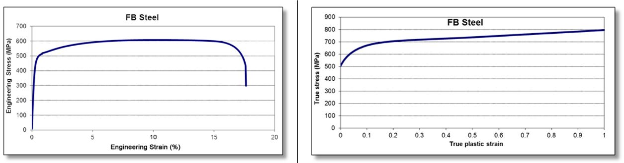
Figure 4: Engineering stress-strain (left graphic) and true stress-strain (right graphic) curve for FB 450/600.T-10
Examples of typical automotive applications benefitting from these high strength highly formable grades include automotive chassis and suspension parts such as upper and lower control arms, longitudinal beams, seat cross members, rear twist beams, engine sub-frames and wheels.
Some of the specifications describing uncoated hot rolled 1st Generation ferrite-bainite (FB) steel are included below, with the grades typically listed in order of increasing minimum tensile strength and ductility. Different specifications may exist which describe uncoated or coated versions of these grades. Many automakers have proprietary specifications which encompass their requirements.
- EN 10338, with the terms HDT450F and HDT580F D-18
- VDA239-100, with the terms HR300Y450T-FB, HR440Y580T-FB, and HR600Y780T-FB V-3
- JFS A2001, with the terms JSC440A and JSC590AJ-23
Formability, true fracture strain
topofpage
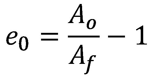
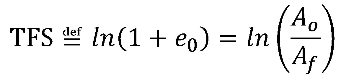
Fracture strain values derived from standard uniaxial tension tests can be used to evaluate automotive crashworthiness and forming behavior of aluminum alloys and Advanced High-Strength Steels (AHSS).Y-10, W-24, W-25, L-22, L-23, T-22, H-15, L-24 The true fracture strain (TFS) and similar concepts have emerged recently as intrinsic measures of local formability for AHSS. TFS is the true (logarithmic) strain associated with the “zero-gage-length” elongation at fracture (e0), where e0 is a conceptual engineering strain value based on an infinitesimal gage length in a tension test, where:
|
Equation 1 |
and Ao and Af are the cross-section area before testing and the fracture area after testing, respectively (constant volume assumed).D-13 It follows that TFS is defined as:
 |
Equation 2 |
TFS is related to percent reduction of area at fracture (Z, %), where:
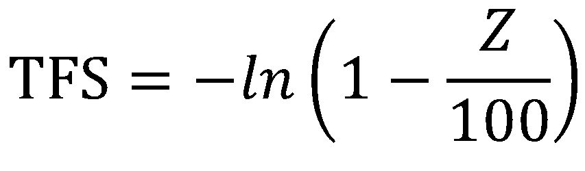 |
Equation 3 |
True Fracture Strain (TFS) Measurement Methods:
Fracture Area (Af)
Tensile test samples have a rectangular cross section before testing, indicated in the left image in Figure 1. The right image shows an idealized tension test specimen fracture surface, where five thickness measurement locations are indicated: two at the edges (ta, te); one at the center (tc), and two at the quarter-width positions (tb, td). Measured approximately at mid-thickness, wf is the fracture width. The dashed outline indicates the original specimen cross-section before testing (to·wo = Ao), and a 10-sided polygon (decagon) approximates the projected fracture area (Af), where the corners of the polygon correspond width-wise to the five thickness measurement locations.
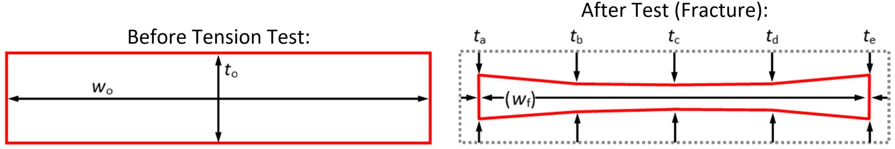
Figure 1: Schematic representation of a tension test specimen before testing (left) and after fracture (right) viewed along the tensile axis.
From the dimensions portrayed in Figure 1, four possible methods to determine Af are indicated in Table 1—three lineal methods and one areal method.H-17 Method A uses a single thickness measurement at mid-width. Alternatively, for Method A the minimum thickness (tmin) may be used in cases where tc ≠ tmin. Method B uses a weighted three-thickness average A-24 —also known as the ASTM parabolic method.H-14, H-16 Method C uses a five-thickness average. For Method D, Af is the area of the polygon depicted in the left image of Figure 1.
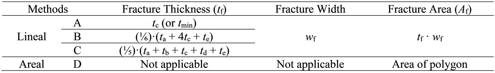
Table 1. Fracture Area Measurement Methods.H-17
Dimensional measurements may be made quickly and conveniently with a calibrated digital microscope equipped with focal stacking capability and linked to image analysis software. Note that tf, wf and Af are respectively: the projected thickness, the projected width, and the projected area of the fracture surface. That is, to accommodate irregular and angled fracture surface features, measurements are made with respect to a virtual plane normal to the tensile axis. Alternatively, lineal measurements may be made with a conventional microscope equipped with a dial indicator or measuring stage. In this case, continual manual refocusing may be necessary to ensure true projected dimensional measurements.
Recently the effects of fracture area measurement method and tension test specimen type on fracture strain values were evaluated H-17. It was concluded that specimen type (i.e., width-to-thickness ratio) has a far greater impact on the consequent fracture strain value in contrast to that of measurement method. It was also advised that, when reporting fracture strain values derived from tension tests, the specimen type, the material thickness, and the fracture area measurement method be clearly indicated.
True Fracture Strain (TFS) Measurement Methods:
Fracture Types
Based solely on fracture appearance, various fracture types may be observed, with examples shown in Figure 2. H-17 The fracture type changes from Type 1 to Type 2 to Type 3 as the tension test specimen width-to-thickness ratio (wo/to) increases (left to right). Type 1 fracture is perpendicular to the tensile axis across the specimen width; Type 2 fracture is an irregular transition from Type 1 fracture to Type 3 fracture; and Type 3 fracture is aligned at an angle across the specimen width (~50-60° from the tensile axis).

Figure 2: Various fracture types observed in uniaxial tension testing, from left to right: Type 1 fracture (wo/to = 4.5—ASTM Standard Sub-size specimen); Type 2 fracture (wo/to = 12.8—ASTM Standard specimen); and Type 3 fracture (wo/to = 16.8—JIS No. 5 Standard specimen); The original width-to-thickness ratio (wo/to) is measured within the gage section of the test specimen.H-17
A similar fracture orientation dependence on specimen width was reported for Dual Phase (DP) steels more than thirty years ago by researchers at the Colorado School of Mines.S-49 A 2018 publication W-23 confirmed this behavior for other AHSS types, and illustrated that the transitional behavior—in terms of critical width-to-thickness ratio—is material dependent.
Figure 3 shows example Type 1 and Type 3 fractures in cross-section at the mid-width position (corresponding to position tc in Figure 1). Type 1 fractures typically run at an angle through thickness (~50-55° from the tensile axis). While most Type 1 fractures resemble that shown in Figure 2 (left) and that shown in Figure 3a, occasional through-thickness chevron profiles and “cup and cone” W-23 type fractures have been observed for Type 1 fractures. Nevertheless, Type 1 fractures are roughly symmetric about a plane normal to the sheet surface at the mid-width position.
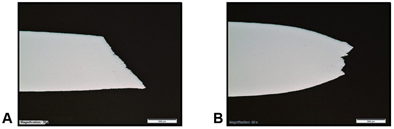
Figure 3. Examples of (A) Type 1 fracture, and (B) Type 3 fracture; Polished through-thickness cross-sections at the mid-width position; Tensile axis is horizontal.
Type 3 fractures invariably show localized necking in through-thickness cross-section as in Figure 3b. Therefore, Type 3 fractures are roughly symmetric about a plane parallel to the sheet surface at the mid-thickness position. Type 2 fractures have both Type 1 and Type 3 characteristics at different positions across the width and thus have no overall plane of symmetry. Various degrees of damage (void formation) are observed in through-thickness cross-sections of fractured specimens— for example, Figure 3. Citation H-18 contains a detailed compendium with more information on this topic.
ElsewhereW-23, L-21 it was explained that the idealized fracture thickness profile—as depicted in the right image in Figure 1—is applicable only to smaller width-to-thickness ratios (thicker, hot-rolled materials or narrower gage sections). For thinner, cold-rolled materials, or for wider gage sections, there is often no clear fracture thickness minimum at the mid-width position. In fact, in some cases a fracture thickness maximum at mid-width has been observed. Furthermore, occasional mid-thickness delamination renders the volume-constancy assumption in question, with associated implications in Equation 1
Formability Classification and Rating System
In 2016 the foundation for a formability classification and rating system was introduced for AHSSH-14, where formability performance expectations are distinguished by the relationships between true fracture strain (TFS) and true uniform strain in a tension test. Such performance mapping concepts continue to be explored and modified by steelmakersH-16, W-23, L-21, D-12, W-22, V-5, R-6, S-48 by automakersH-18, H-19 and by international industry consortiums.G-20 Traditionally AHSS performance has been represented by the product of ultimate tensile strength and total elongation (UTS x TE) and relative position on the so-called “banana diagram” or Global Formability Diagram. While this conventional methodology discriminates behavioral extremes, much is lost regarding the nuances of local formability.
Intrinsic Formability Parameters
Widely considered an intrinsic measure of global formability, the true uniform strain (εu) is the logarithmic strain associated with uniform elongation (UE, %) in a uniaxial tension test, where:
 |
Equation 4 |
Example TFS and εu values are shown for a series of 980-class AHSS (980 MPa minimum tensile strength) in Figure 4H-14. In this analysis, TFS values ranged from less than 0.5 [DP 980 (LSi)] to more than 1.0 (CP 980), and εu values ranged from 0.05 (CP 980) to 0.15 (GEN3 980). The Third Generation AHSS materials (GEN3-type) have the largest εu values, and the Multi-Phase/Complex-Phase steels (MP/CP-type) have the largest TFS values. As a group the Dual Phase steels (DP-type) have intermediate εu values and a wide range of TFS values. As illustrated in Figure 4, TFS is far greater than εu. A similar disparity between fracture strain and uniform strain was shown in Citation D-14, and no consistent relationship between the two parameters was determined.

Figure 4: True uniform strain (εu) and true fracture strain (TFS) values for a series of 980-class AHSS; Error bars show the range among three test specimens for each material.H-14
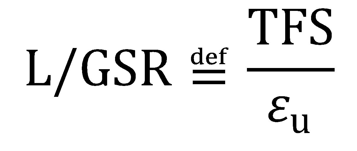
The local/global strain ratio (L/GSR) and the formability index are key parameters to guide application-specific material selection and to help set targets for future AHSS grade developments.H-14, H-16 The L/GSR reflects the relative preponderance of local formability to global formability and is defined as:
 |
Equation 5 |
The L/GSR is useful in understanding relative intrinsic formability “character”. Materials with higher relative TFS values are naturally expected to perform better under flanging, edge stretching and tight-radius bending conditions [e.g., MP 980 (LCE) and CP 980 in Figure 4], while materials with higher relative uniform strain values (i.e., higher terminal n values) are better suited for stretch forming and are able to distribute strain more uniformly (e.g., GEN3 980 and GEN3 980-HY in Figure 4).
Furthermore, the formability index (F.I. in the formula) is defined as:
 |
Equation 6 |
This index represents an intermediate strain value between εu and TFS and provides a convenient measure of the overall formability expectation, where both local formability and global formability are considered. As an example, Figure 5 shows an exponential relationship between F.I., and the limiting bend ratio (r/t) determined from 90° V-bend testing for the same series of 980-class AHSS represented in Figure 4.H-14 It was reasoned that in the early stages of deformation, global formability (εu) dictates the strain distribution around the punch nose, while fracture resistance is governed by local formability (TFS) in the latter stages of deformation.

Figure 5. Correlation between the limiting bend ratio (f) and the formability index (F.I.) for a series of 980-class AHSS. A higher formability index corresponds to a lower (better) limiting bend ratio in 90° V-bend testing.H-14
Local/Global Formability Map
Figure 6 illustrates the essential framework of the local/global formability map—known eponymously as the Hance diagram.H-14, D-12, G-20 Here, the dashed lines represent the boundaries between global character (L/GSR < 5), balanced character (5 < L/GSR < 10), and local character (L/GSR > 10). The continuous curves represent arbitrary iso-F.I. contours corresponding to the values indicated (in parentheses). The qualitative assessments (Poor through Excellent) indicated for each formability level are also arbitrary; however, these performance level monikers were chosen to reflect real-world experience. Portrayed in this way (in contrast to Figure 4, for example), the relationships between true fracture strain and true uniform strain are more discernable, and both the formability character and the formability level become apparent.

Figure 6: Essential framework of the local/global formability map concept.H-16
Case Study Using the Local/Global Formability MapH-15
The basic utility of the local/global formability map concept was demonstrated for an automotive seating system development program.H-15 In this case study, stamping trials were conducted with two 980-class AHSS (980 MPa minimum UTS designation):
- 1.6mm 980DP(LSi): A classic Dual Phase (DP) ferrite/martensite steel with low silicon content (LSi), and
- 1.6mm 980MP(LCE)—a Multi-Phase (MP) steel with high yield strength and low carbon equivalent (LCE).
Basic formability parameters are summarized in Table 2 for the trial materials. Based solely on elongation values (UE, TE), one might have concluded that the formability of 980DP(LSi) would exceed that of 980MP(LCE).
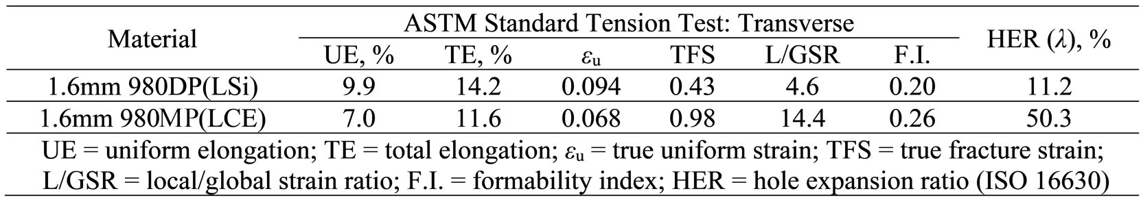
Table 2. Formability Parameters for Two 980-Class AHSS.
However, the stamping trial results were counterintuitive and drastically different among the two trial materials. The 980DP(LSi) material exhibited severe edge-cracking in multiple locations, while the 980MP(LCE) material ran without issue. Both materials were free of necking-type failures as predicted by computer simulations (sufficient global formability). An example part overview is shown in Figure 7. Typical 980DP(LSi) edge cracks are shown in Figure 8 for a pierced/extruded hole (Location 1) and for a blanked/stretched perimetric edge (Location 2). Clearly, relative sheared-edge ductility may not simply be deduced from conventional tensile elongation values.
![Figure 7: Overview of a stamped automotive seating component [length ~ 480 mm (19 in.)]. H-15](https://ahssinsights.org/wp-content/uploads/2020/10/2.3.5a-Figure7.svg)
Figure 7: Overview of a stamped automotive seating component [length ~ 480 mm (19 in.)].H-15
![Figure 8: Close-up views of Location 1 (left) and Location 2 (right) identified in Figure 7 [material: 980DP(LSi)]; Location 1 is a pierced hole that was extruded during forming, and Location 2 is a blanked perimetric edge that was stretched during forming (underside with respect to Figure 7). H-15](https://ahssinsights.org/wp-content/uploads/2020/10/2.3.5-Fig8.jpg)
Figure 8: Close-up views of Location 1 (left) and Location 2 (right) identified in Figure 7 [material: 980DP(LSi)]; Location 1 is a pierced hole that was extruded during forming, and Location 2 is a blanked perimetric edge that was stretched during forming (underside with respect to Figure 7).H-15
The local/global formability map coordinates of the 980DP(LSi) and 980MP(LCE) trial materials are shown in Figure 9. With reference to the framework described in Figure 6, 980DP(LSi) exhibits global/balanced character with an overall borderline rating of Fair/Good (F.I. = 0.20); while 980MP(LCE) has decidedly local character with an overall rating of Good (F.I. = 0.26). Furthermore, the TFS value of 980MP(LCE) is more than twice that of 980DP(LSi).

Figure 9: Local/global formability map featuring three 980-class AHSS—980DP(LSi), a classic DP ferrite/martensite steel with low silicon content (LSi); 980MP(LCE), an MP steel with high yield strength and low carbon equivalent (LCE); and 980GEN3, a third generation AHSS. Image based on Citations H-15 and H-17.
As an independent confirmation of the local formability advantage of 980MP(LCE), the hole expansion ratio (HER, λ) is more than four times that of 980DP(LSi) (Table 2). A strong correlation between TFS and λ has been confirmed by several authors L-22 L-23 T-22 H-15 As the component featured in this case study is dominated by extremely challenging edge-stretching conditions, 980MP(LCE) is the clear wiser material selection. However, in applications with more demanding global formability requirements, other issues such as intolerable strain localization could arise, and a third generation AHSS might be the best choice. As an example, when contrasting 980GEN3 AHSS (third generation AHSS) to 980DP(LSi) in Figure 9, the intrinsic global and local formability parameters (εu and TFS), as well as the F.I, are approximately 50% greater.
True Fracture Strain (TFS): Alternatives to TFS
While the local/global formability map methodology was developed in the context of true fracture strain (TFS), there are other ways to represent intrinsic local formability (fracture resistance) with data derived from standard uniaxial tension tests. In the original conception (Hance diagram), true uniform strain (εu) and TFS are two points along a logarithmic strain continuum from zero to fracture, and the relationships between these values elegantly describe the formability character (local/global strain ratio) and the overall formability level (formability index). The “best” local formability parameter may be a matter of practicality or applicability, or simply a matter of preference. Each method has its strengths and weaknesses, and such fracture strain concepts continue to evolve.
True Thinning Strain at Fracture
The true fracture strain (TFS) value is an area-based measurement of fracture strain and thus reflects the tension test specimen width change as well as the thickness change, for better or for worse. Citation H-18 suggests that the true thinning strain at fracture (ε3f) is a more appropriate measure of local formability, where:
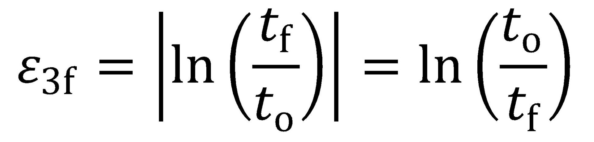 |
Equation 7 |
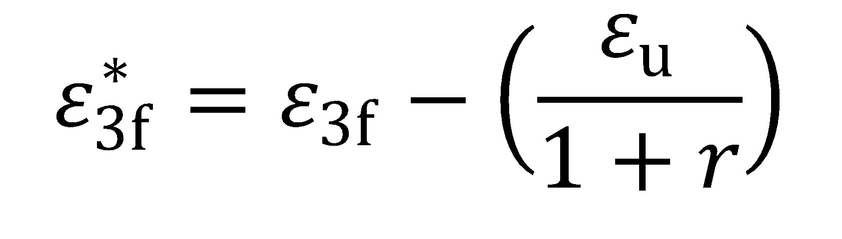
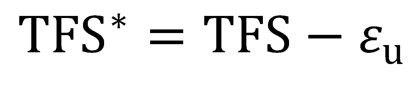
and to and tf are the original thickness (before testing) and final thickness (after fracture). By convention ε3f is a positive value and represents the absolute value of the true thickness strain at fracture (a negative value). Furthermore, the post-uniform portion of the fracture strain may be isolated by subtracting the uniform component of thinning strain, where:
 |
Equation 8 |
and εu and r are the true axial uniform strain and the plastic strain ratio (normal anisotropy) measured during the tension test, respectively. Post-uniform fracture strain components might be more relevant to materials with high uniform elongation values such as TWIP steels H-18. In a similar way, the post-uniform portion of the area-based TFS value may be expressed as:
 |
Equation 9 |
Another study W-23 concluded that: (1) area-based fracture strain measurements such as TFS result in less experimental scatter when compared to thickness-based fracture strain measurements such as ε3f, and (2) area-based measurements show less dependence upon the method by which fracture strains are determined. It appears that a single thickness measurement may misrepresent the fracture strain and that a multiple-thickness (average thickness) or area measurement approach may be more stable.
Critical Fracture Strain
Perhaps a lesser-known and under-exploited representation of fracture strain is the so-called critical fracture strain value (CFS)—introduced in 1999 for aluminum alloys in Citation Y-10 and re-visited in 2007 in the context of High-Strength Steel in Citation W-24. In concept CFS is the estimated true thinning strain at fracture, where:
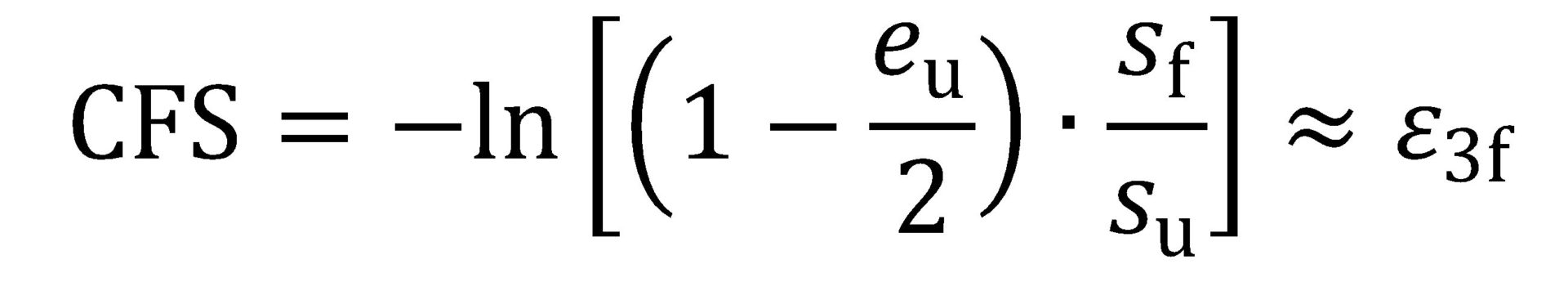 |
Equation 10 |
In determining CFS, only the engineering stress-strain data from a uniaxial tension test are needed—that is, no post-fracture area or thickness measurements are required: eu is the engineering uniform strain value (% uniform elongation/100); sf is the engineering fracture stress; and su is the ultimate tensile strength or UTS. Figure 10 shows an example engineering stress-strain curve for a 980-class AHSS, where the parameters relevant to CFS are marked. In this example, CFS = -ln[(1-0.07/2)·(787/1015)] = 0.29.

Figure 10: Example engineering stress-strain curve for a 980-class AHSS. Here, eu is the engineering uniform strain, su is the ultimate tensile strength (UTS), sf is the engineering fracture stress, CFS is the critical fracture strain, and ε3f is the true thinning strain at fracture.
True Fracture Strain (TFS):
Correlation to Hole Expansion Ratio
In a recent studyL-5, tensile properties (80 mm gage length) and hole expansion ratio were measure for AHSS with minimum tensile strength designations ranging from 600 to 1200 MPa, and thickness between 1 and 2 mm. No particular correlation was found between the hole expansion ratio and conventional tensile properties such as uniform elongation, total elongation, n-value, and so on.
The most promising relationship was found between the hole expansion ratio (converted to logarithmic strain) and the true thinning strain at fracture in tension. This relationship is illustrated in Figure 11 for total thinning strain (ε3f, Equation 7) on the left, and for post-uniform thinning strain (ε*3f, Equation 8) on the right. In both cases, better correlation is shown for transverse tension tests rather than for longitudinal tension tests (linear fit through the origin).

Figure 11: Hole expansion ratio (logarithmic strain) as a function of true thinning strain at fracture. Left graph: total thinning strain (ε3f); Right graph: post-uniform thinning strain (ε*3f).L-5
While the above correlations are good, the inherent scatter associated with the hole expansion test, fracture strain measurements, and other local formability parameters may limit applicability in a production environment. Furthermore, various factors affect hole expansion in production environments, including hole preparation technique, edge condition, and cutting clearance.
 |
Thanks are given to Brandon Hance, Ph.D., who contributed this article. |


![Figure 7: Overview of a stamped automotive seating component [length ~ 480 mm (19 in.)]. H-15](http://ahssinsights.org/wp-content/uploads/2020/10/2.3.5a-Figure7.svg)
![Figure 8: Close-up views of Location 1 (left) and Location 2 (right) identified in Figure 7 [material: 980DP(LSi)]; Location 1 is a pierced hole that was extruded during forming, and Location 2 is a blanked perimetric edge that was stretched during forming (underside with respect to Figure 7). H-15](http://ahssinsights.org/wp-content/uploads/2020/10/2.3.5-Fig8.jpg)


