High Strain Rate Testing
Highlights of this page are summarized in the video below, but we encourage you to read more for a deeper understanding.
Background and Motivation
As more companies aim to reduce their product’s time to market, research and design engineers have begun integrating predictive modeling into their process. These models, whether finite element based or artificial intelligence based, all rely on quality mechanical testing results. Companies within the automotive industry have seen that accurately predicting large scale tests such as crashworthiness trials can greatly expedite the time it takes to get their products to market. One of the more important details in predicting these expensive and time-consuming tests is to understand how the materials within the design are affected by the higher rates of deformation or their strain rates.
From an application standpoint, the ultimate goal of high strain rate characterization is to enable accurate prediction of component-level and system-level crash behavior. For example, in a frontal collision, the progressive folding of a front rail or crash box depends on the dynamic flow stress of the steel, as well as its strain hardening and failure characteristics. Similarly, side-impact performance is heavily influenced by the behavior of B-pillar reinforcements under high-rate loading. Without accurate high strain rate data, simulations may underpredict or overpredict intrusion, energy absorption, and failure, leading to suboptimal designs or costly physical test iterations.
Traditional standardized tensile tests have been used for over a century – ASTM E8 was first approved in 1924. Testing laboratories using standards like ASTM E8, ISO 6892-1, and JIS Z-2241 produce repeatable and reproducible mechanical properties for metals undergoing tensile deformation, but each of these standards requires the test to be run at a speed orders of magnitude lower than those occurring during events like sheet metal forming and automotive crash. A tensile test run according to ASTM E8 to obtain the yield properties of a metal is run at a strain rate of 0.00035 strain per second (0.00035/s). For comparison, a stamping process has strain rates on the order of 1 to 10 strain per second, and an automotive crash can have strain rates up to 1,000 strain per second (Figure 1).
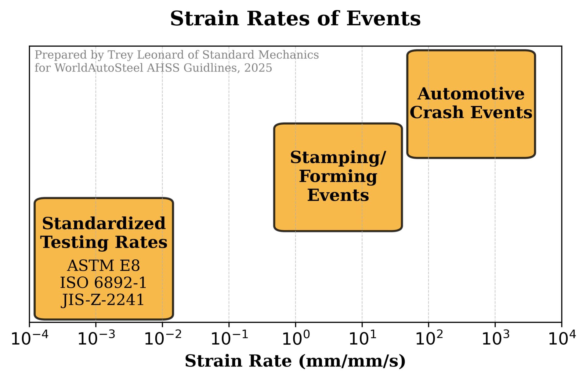
Figure 1. Strain rates of different events.
Historically, no guidelines have been available as to the testing method to obtain high strain rate mechanical properties. Decisions on specimen dimensions, measurement devices, and other important issues which are critical to the quality of testing results were made within each individual laboratory. As a result, data from different laboratories were often not directly comparable. A WorldAutoSteel committee evaluated various procedures, conducted several round-robins, and developed a recommended procedure, which evolved into what are now the first two parts of ISO 26203, linked below.
Published standards addressing tensile testing at high strain rates include:
- International Organization for Standardization (ISO), “ISO 26203-1: Metallic materials — Tensile testing at high strain rates — Part 1: Elastic-bar-type systems.”
- International Organization for Standardization (ISO), “ISO 26203-2: Metallic materials — Tensile testing at high strain rates — Part 2: Servo-hydraulic and other test systems.”
- Stahl-Eisen-Prüfblätter (SEP) Standard, “SEP 1230: The Determination of the Mechanical Properties of Sheet Metal at High Strain Rates in High-Speed Tensile Tests.”
Standardization efforts, such as those related to ISO 26203, have helped bring consistency to high strain rate tensile testing, but variability still exists across laboratories. Many factors contribute to these variances: unstandardized specimen geometries and gripping methods, variances in specimen loading conditions, lower quality strain measurement techniques, and non-optimized fixturing for wave transmission and measuring. For automotive applications, this variance places a premium on internal validation—correlating material test data with component-level crash tests to ensure that the material model behaves correctly within the simulation environment.
Strain Rate Sensitivity
Steel alloys typically possess positive strain rate sensitivity, or m-value when tested at ambient temperature, meaning that strength increases with strain rate. This has benefits related to improved crash energy absorption.
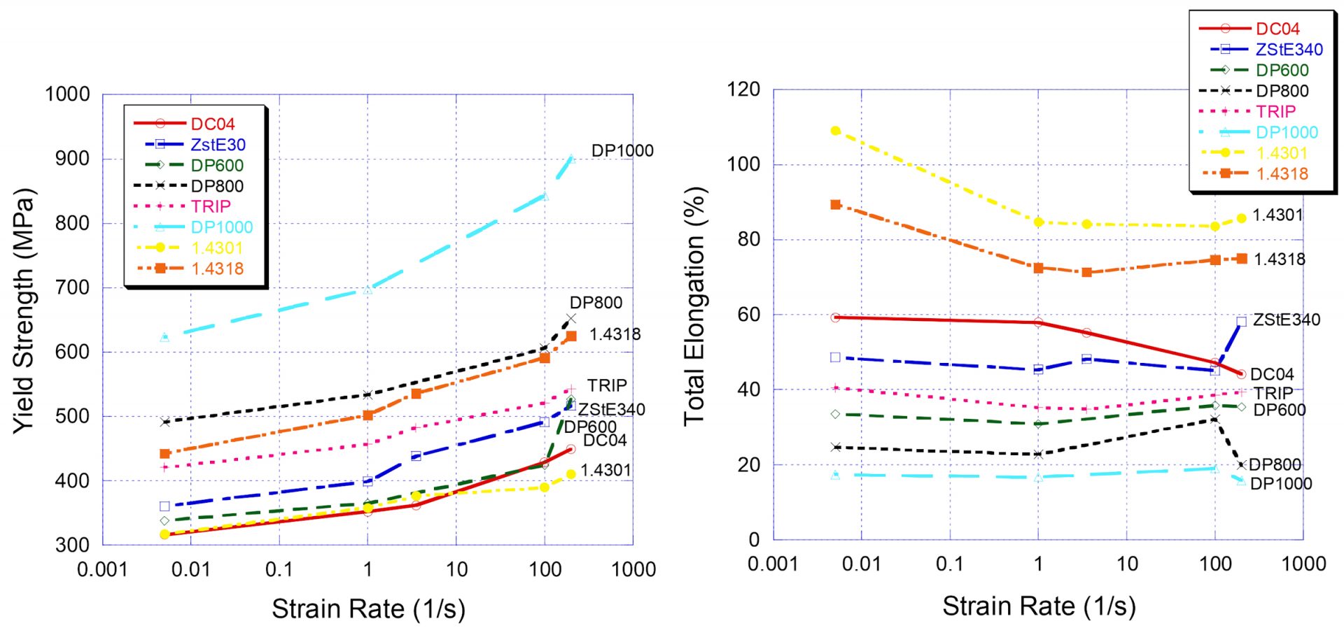
The specific response as a function of strain rate is grade dependent. Some grades get stronger and more ductile as the strain rate increases (left image in Figure 2), while other grades see primarily a strength increase (right image in Figure 2). Increases are not linear or consistent with strain rate, so simply scaling the response from conventional quasi-static testing does not work well. Strain hardening (n-value) also changes with speed in some grades, as suggested by the different slopes in the right image of Figure 2. Accurate crash models must also consider how strain rate sensitivity impacts bake hardenability and the magnitude of the TRIP effect, both of which are further complicated by the strain levels in the part from stamping.

Figure 2: Two steels with different strength/ductility response to increasing strain rate.A-7
Modeling Strain Rate Sensitivity — Cowper-Symonds vs. Johnson-Cook
Knowing that the strain rate directly affects mechanical properties, many automotive OEMs and suppliers generate stress-strain curves across a range of strain rates, typically spanning quasi-static (~10⁻⁴ s⁻¹), intermediate (~1 to 10² s⁻¹), and high-rate (~10² to 10³ s⁻¹) regimes. These datasets are then used to calibrate constitutive models implemented in crash simulation software such as LS-DYNA or Abaqus.
Models like Cowper–Symonds or Johnson–Cook incorporate strain rate terms that predict the increase in strength of a material deformed at a higher strain rate, but their predictive capability depends entirely on the quality and range of the underlying experimental data, as well as the assumptions incorporated into the model such as the strain range. Figures 3, 4, and 5 show that the Cowper–Symonds model does a better job than the Johnson–Cook model when considering the strain rates associated with vehicle crash.
The Cowper-Symonds model can be written as:
Equation 1
where σd is the strength of the material at a strain rate έ, σs is the strength of the material at a theoretical strain rate of zero strain per second, and C and p are model parameters.
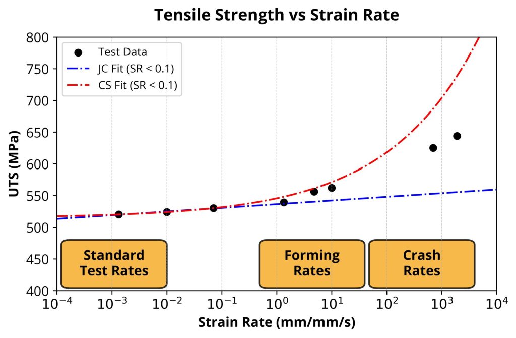
Figure 3. Cowper-Symonds and Johnson-Cook Strain Rate Sensitivity Model fit to Low-Rate Experimental Data
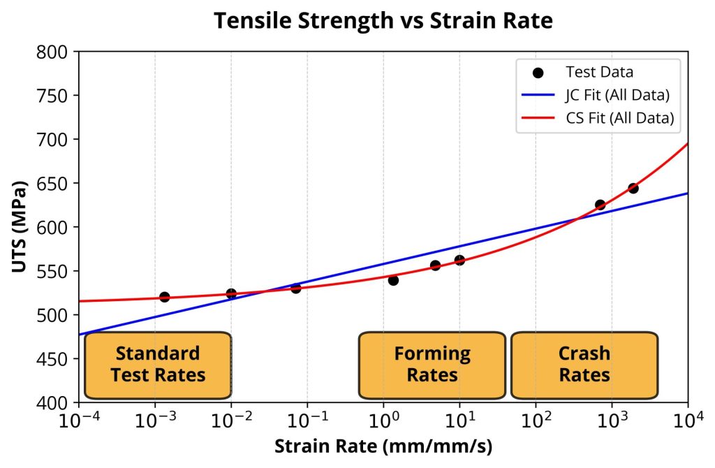
Figure 4. Cowper-Symonds and Johnson-Cook Strain Rate Sensitivity Model fit to All Experimental Data
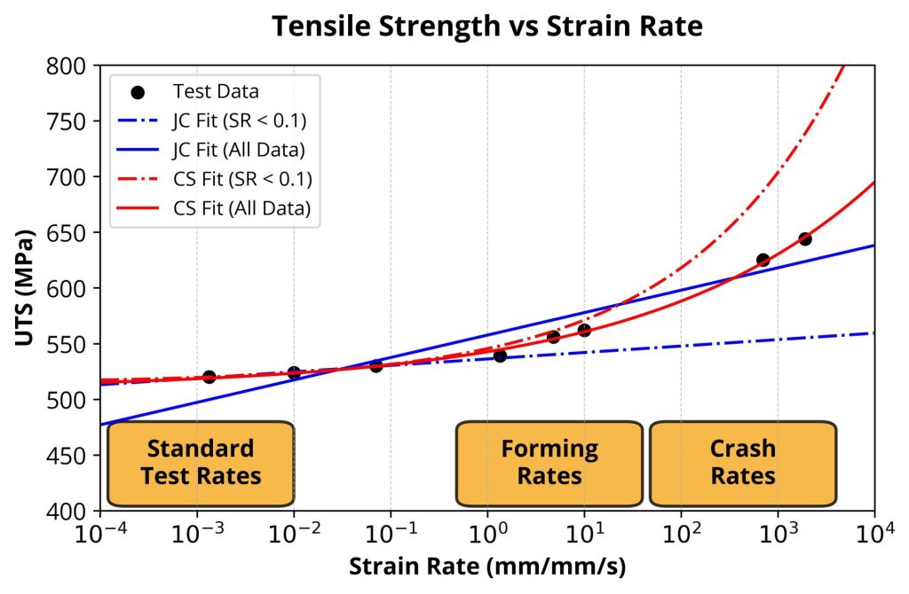
Figure 5. Cowper-Symonds and Johnson-Cook Strain Rate Sensitivity Model fit to Low-Rate and All Experimental Data
Figure 6 shows two best fit curves for this Cowper-Symonds model to the tensile strengths of a cold rolled steel across a range of strain rates. The first considers only data that can be obtained using traditional tensile testing machines (strain rates less than 0.1 strain per second) while the second uses data up to 2,000 strain per second. Both models have minimal errors at strain rates below 0.1 strain per second, but as the limited model begins to extrapolate data beyond this strain rate regime, the associated error begins to grow exponentially causing large errors at the strain rates typical in crashes.
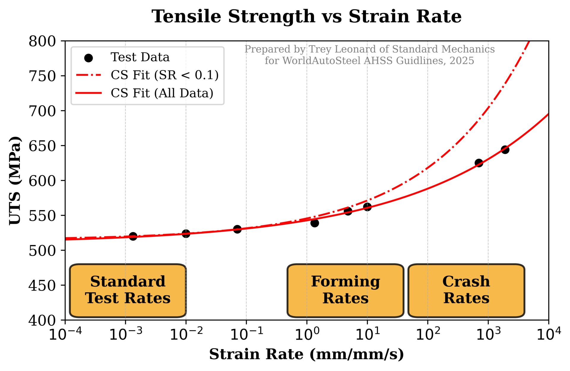
Figure 6. Example of extrapolation of tensile strength vs strain rate data using a Cowper-Symonds model. The dashed curve is an extrapolation based only on data acquired using traditional tensile testing machines, where strain rates are less than 0.1 strain per second. The solid curve is the extrapolation when considering data from equipment capable of achieving 2,000 strain per second.
Testing Methods and Equipment
The biggest obstacle to measuring how a material responds to different strain rates is that it requires several different types of equipment. This is due to the need to run tests at up to six or seven different orders of magnitude to fully characterize the material. Figure 7 shows which mechanical testing equipment is most used to perform tensile tests based on the strain rate of the test. A broader range of testing methods for more strain rates can be found in the ASM Handbook, Volume 8: Mechanical Testing and Evaluation.A-88 The limits for the strain rate range that each type of test equipment can achieve varies based on the design and attributes of each specific machine as well as the specimen geometry used in testing. In tensile and compression testing, going from a longer specimen to a shorter specimen allows for a specific machine to increase its upper limit on strain rates.
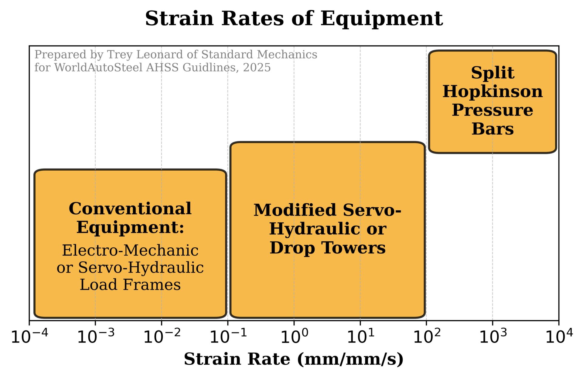
Figure 7. Testing equipment most used to test materials at strain rates between 0.0001 strain per second and 10,000 strain per second in uniaxial tension.
Modified Servo-Hydraulic Machines
Modified servo-hydraulic testing machines are specifically engineered to characterize the dynamic mechanical properties of materials at high strain rates, often reaching strain rates up to 500 strain per second. Unlike conventional servo-hydraulic machines, which used closed-loop control for precise lower-speed testing, these modified systems incorporate design features that overcome the limitations of standard hydraulic controls at higher speeds. Many of these machines utilize extreme high flow valves along with slack adapters. The higher flow valves allow for higher accelerations while the slack adapters decouple the actuator from the specimen while the actuator accelerates to a desired test speed.
Split Hopkinson Pressure Bars
A split Hopkinson pressure bar (sometimes referred to as Kolsky bar or simply SHPB) is an impact-based device that is designed to characterize the dynamic mechanical properties of materials at strain rates above 100/s. The SHPB system uses a striker rod to generate a stress wave which induces plastic deformation in a specimen placed between two elastic bars. The stress wave generated by the striker bar in the first elastic bar (called the incident bar) is measured by a strain gauge fixed at the midpoint of the incident bar. When the stress wave reaches the specimen, part of the stress wave is transmitted through the specimen into the second elastic bar (called the transmitted bar) where it is measured by a second strain gauge. The rest of the stress wave is reflected off the specimen and returns down the incident bar to be re-measured by the strain gauge. Figure 8 shows how the stress waves propagate through a SHPB system during a compression test. There are various options to modify the compression SHPB setup to run a tensile test, but the most common is to replace the striker bar with a tube that slides on the incident bar where it impacts a flange on the end of the incident bar causing a tensile stress wave to propagate towards the specimen instead of a compression wave.
split Hopkinson pressure bar system during a high strain rate compression test.
High Strain Rate Testing Challenges
Many other challenges complicate testing materials at higher strain rates. Three of the major challenges are
- Challenges of measuring strain at high speeds
- Challenges of accounting for inertial effects
- Challenges of accounting for adiabatic heating
Strain Measurements in High Strain Rate Testing
During standardized mechanical testing, clip-on extensometers and deflectometers provide excellent extension measurements. As the speed of the test increases, the mass of the extensometer inhibits its use due to slippage of the contact points or interference with the specimen, both of which lead to erroneous test results and potential damage to the device. During high strain rate tests, the simplest means of measuring specimen displacements is to derive them based on the stress waves from the test. A detailed derivation of this method can be found here. This method works well for compression testing, but during tensile testing, events such as slippage of the specimen within the grips or deformation of the radius section of the specimen add to the displacements of the test. These additional displacements overshoot the tensile strain of a specimen during the test. This has led to the nearly universal adoption of optical strain measurements for high strain rate tension tests.
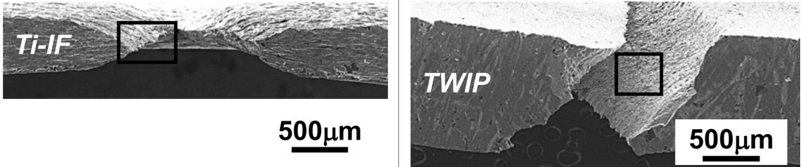
The most common optical method is digital image correlation (DIC). DIC correlates a series of images taken during the deformation of a specimen and calculates the corresponding strains of the specimen. It does this by tracking a black-and-white speckle pattern painted on the specimen’s surface which creates a series of high-contrast features as shown in Figure 9.
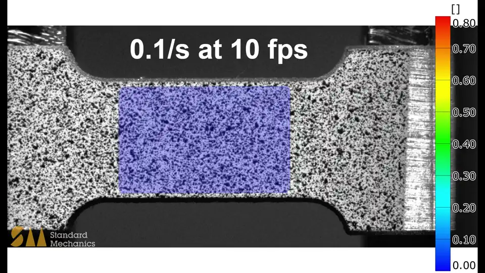
Figure 9. Two examples of 2D digital image correlation (DIC) showing the true equivalent strain fields during tensile tests performed at 0.1 strain per second and 1000 strain per second.
When testing round or more complex specimens, two cameras are required to track the surface of the specimen in three-dimensional space. This is referred to as 3D DIC, and it often requires more rigorous calibration for use in testing due to its multi-camera complexity. Alternatively, there are a series of one-dimensional options for strain measurements. The simplest utilizes a high-speed line scan camera to measure the displacement of a specimen along the test direction. While the two- and three-dimensional approaches bring in more data, the one-dimensional approach has been shown to provide excellent resolution at a lower adoption cost.Z-16
Accounting for Inertia in High Strain Rate Testing
At strain rates around one to ten strain per second, inertial effects can begin to complicate the interpretation of test results. These effects can be broken into two varieties: inertia of the specimen being tested and inertia of the equipment being used. Both directly affect the load values measured during a given test. In a modified servo-hydraulic load frame, large grips can create a large difference in stiffness (known more specifically as mechanical impedance) between each grip and the specimen. This difference causes more of any generated stress wave to be reflected at the interface as opposed to transmitting through; thus, as the wave travels back-and-forth through the specimen, the load it experiences “rings up”. This is sometimes referred to as “load ringing”. During this transient period of ring-up, the wave is amplifying or changing shape each time it reaches an end of the specimen. From this, the specimen experiences a load gradient across its gauge section depending on where the wave is at that point. After a certain number of reflections have occurred, the stress wave within the specimen becomes uniform and the specimen is determined to be in stress equilibrium. The number of oscillations it takes for this to occur is greatly dependent on the maximum frequency of the stress wave that enters the specimen and the ratio of mechanical impedances between the specimen and its grips. The lower the difference in impedances, the lower the energy that is reflected back into the specimen. The overall time of this period is not affected by the strain rate of the test being performed. This is because the phenomenon is based more so on the number of times the wave traverses the specimen which is solely dependent on the wave speed and length of the specimen. The wave speed of a material (assuming one—dimensional wave propagation) is calculated by:
Equation 2
Where c is the wave speed of the material, E is the Young’s modulus of the material, and ρ is its density. When viewing test results, the load ringing can be seen as a decaying sinusoidal that begins when the specimen is first loaded. Figure 10 shows an example of how this could look across various strain rates. Each data set shares the same decay time constant, frequency, and magnitude of oscillations. Holding these three as constant simulates running tensile tests using the same specimen geometry, machine, and grips but varying the strain rate of the test. In the data set at lower strain rates, the effect of load ringing is minor with no notable difference between the actual response and the measured response at 10 strain per second. At 30 and 100 strain per second, the yield portions of the stress-strain curves are noisy, but the overall hardening profile is still clean. At 300 strain per second, the oscillations affect most of the hardening potion of the stress-strain curve. At 1000 strain per second, the overall profile of the stress-strain curve can be made out including strain to failure, but no details regarding hardening, uniform elongation, or tensile strength can be stated without large error bands. At 3000 strain per second, very little can be discerned from the data.
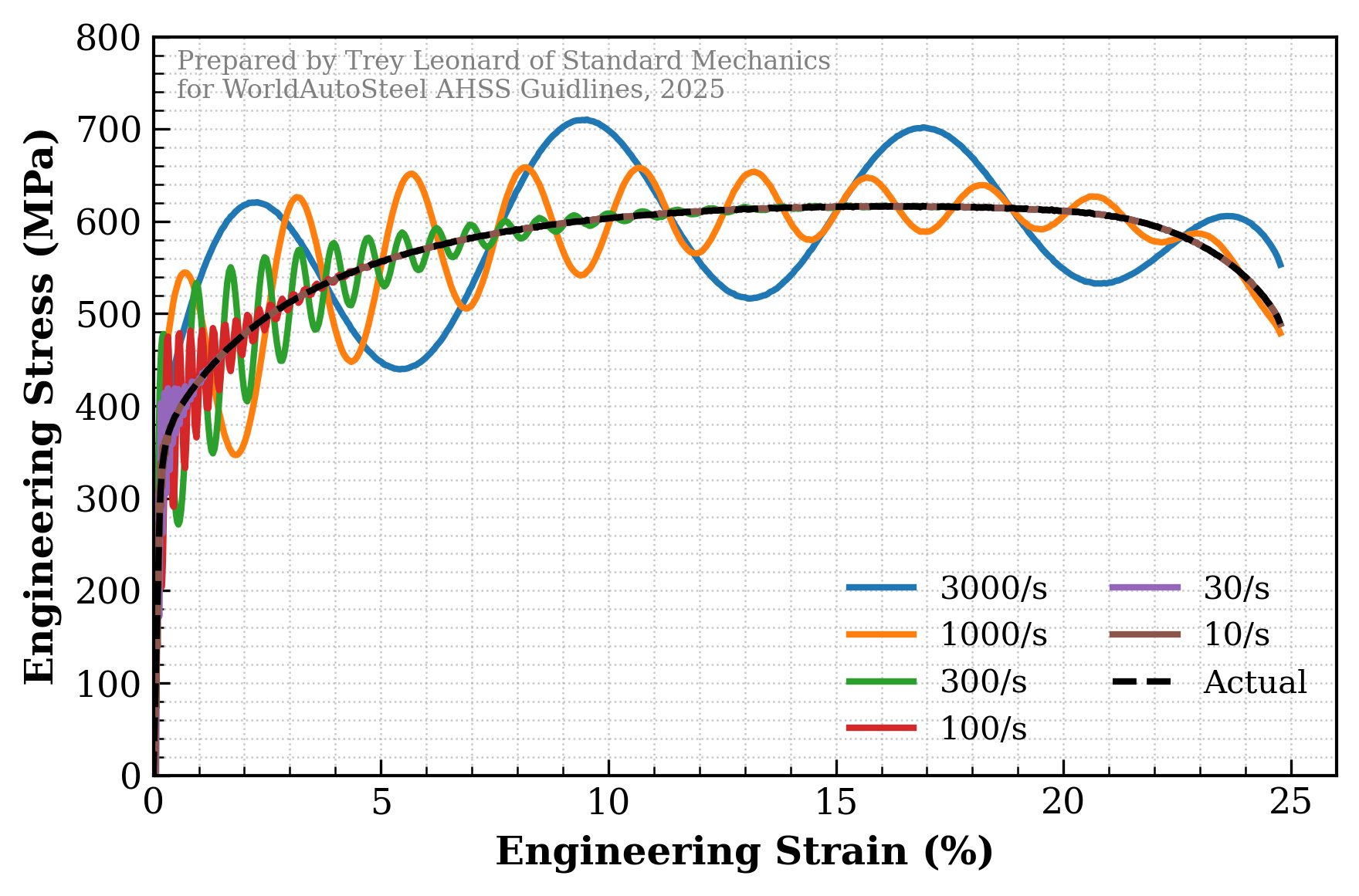
Figure 10. Illustration of theoretical frequency responses of dynamic tensile tests performed at various strain rates. All tests share the same decaying time constant, frequency, and magnitude of oscillations.
Some laboratories have adopted an inverse method that takes data with excessive load ringing and derives a stress-strain model. This is done by simulating the equipment used to perform the test along with the specimen tested in a finite element model. Then, repeated iterations of the stress-strain profile are sequentially optimized until the simulation best fits the data read from the test which includes the load oscillations. While this method has shown great potential, it is often too time intensive and expensive to justify in most industrial applications.
Adiabatic Heating in High Strain Rate Testing
The final challenge when testing materials at high strain rates comes from a by-product of plastic deformation of materials: adiabatic heating. Quasi-static tests allow for iso-thermal testing where the rate of heat being generated from plastically deforming the specimen is exceeded by the rate that heat is lost to the surrounding environment. As the strain rate of the test is increased, so too does the rate of plastic work and heat generation within the specimen. This internal heating is also compounded with the need for high intensity lighting to illuminate any high-speed optical methods for measuring strain of specimens. Because of these heat sources without equivalent cooling, the material response as measured by a high strain rate test is jointly affected by the higher strain rate as well as the elevated temperature of the specimen. These two effects have been shown experimentally to not be independent of one another, further complicating the analysis and interpretation of these tests. More complex multi-physics material models are often employed to account for these coupled effects in finite element model simulations.
Visit our page on high strain rate testing of spot welds to learn more about that application!
 Thanks are given to Trey Leonard, for his contributions to this page. Trey is the founder and CEO of Standard Mechanics, LLC, where he delivers advanced mechanical testing services and solutions across a wide range of applications, from automotive design to consumer electronics. His expertise spans formability, fatigue, and strain rate sensitivity testing. Beyond conducting tests, he partners with customers to ensure the development of high-quality, calibrated material cards and models for accurate finite element simulations. Dr. Leonard earned his Ph.D. in Mechanical Engineering from Mississippi State University, where he pioneered and licensed technologies in dynamic material testing and characterization. Building on this foundation, he continues to develop innovative testing methods and technologies that advance the field of dynamic mechanical testing. He also contributes to the broader engineering community through his work with ASTM International, where he serves on the E28 Committee on Mechanical Testing, regularly reviewing and improving industry standards.