homepage-featured-top, main-blog, News
There is interest in the sheet metal industry on how to adopt Industry 4.0 into their legacy forming practices to significantly improve productivity and product quality. Figure 1 illustrates four important variables influencing part quality: material properties, die friction response, elastic deflection of the tool, and press dynamic characteristics. These variables are usually difficult to measure or track during the production runs. When these variables significantly influence the part quality and the scrap rate increases, the operators manually adjust the forming press parameters (speed and pressure), lubricant amount, and tooling setup. However, these manual adjustments are not always possible or effective and can be costly for the increased part complexity.

Figure 1: Important variables influencing the stamping quality.H-35
The ultimate vision for Industry 4.0 in sheet metal forming is an autonomous forming process with maximum process efficiency and minimum scrap rate. This is very similar to the full self-driving (FSD) vision of the electric vehicle today. This will be valuable for the automotive industry that has to process large production volumes with various steel grades.
For example, normal variations of the incoming material properties for Advanced High-Strength Steel (AHSS) may have a significant effect on part quality associated with necking, wrinkling, and cracking, which in turn drastically increases the production cost. This variation of the incoming material properties increases uncertainty in sheet metal forming by making consistent quality more challenging to achieve, thereby increasing the overall manufacturing cost. A nondestructive evaluation (NDE) can be a useful tool to measure incoming material properties.
There are several types of NDE sensors. Most of the sensors need further development or are not suitable for production applications. However, some of the NDE sensors, such as the eddy current tools, laser triangulation sensors equipment, and equipment developed by Fraunhofer IZFP called 3MA (micromagnetic, multiparametric microstructure, and stress analysis), have already been applied to a few limited production applications. These sensors can be used to provide data during production to select the optimal parameters. They also can be used to obtain material properties for finite element model (FEM) analysis. Studies in deep drawing of a kitchen sink production used a laser triangulation sensor to measure the sheet thickness and an eddy-current sensor to measure the yield strength, tensile strength, uniform elongation, elongation to break, and grain size of the incoming material. The material data is used as an input for simulations to generate the metamodels to determine the process window, and it is used as an input for the feed-forward control during the process.K-27
Figure 2 shows how NDE tools are used for feed-forward controls and cameras for feedback control to determine the optimum press setting on sink forming production.

Figure 2: Process control for sheet metal forming of kitchen sink production.H-36
Another study proposed the use of Fraunhofer’s 3MA equipment to determine the mechanical properties of incoming blanks for a sheet forming process. The 3MA sensor correlates the magnetic properties of the material with the mechanical properties and calibrates the system with the procedure outlined in Figure 3. The study showed a good correlation between the measurements from the sensor and the tensile testing results; however, the sensor should be calibrated for each material. Also, the study proposed to use a machine-learning algorithm instead of a feed-forward control to predict the most effective parameters during the drawing process.K-28

Figure 3: Calibration procedure for 3MA sensors.K-28
Technologies associated with Industry 4.0 have a natural fit with AHSS. The advanced slide motion capabilities of servo presses combined with active binder force control can be paired with stamping tonnage and edge location measurements from every hit to create closed-loop feedback control. With press hardening steels (PHS), vision sensors and thermal cameras can be used for controlling the press machine and transfer system.
Have a look at the Dr. Kim’s detailed article on Industry 4.0 for more examples of NDE sensors, as well as information on applying Industry 4.0 to forming process controls.
Blog, main-blog, RSW Modelling and Performance
Modelling resistance spot welding can help to understand the process and drive innovation by asking the right questions and giving new viewpoints outside of limited experimental trials. The models can calculate industrial-scale automotive assemblies and allow visualization of the highly dynamic interplay between mechanical forces, electrical currents and thermal flow during welding. Applications of such models allow efficient weldability tests necessary for new material-thickness combinations, thus well-suited for applications involving Advanced High -Strength Steels (AHSS).
Virtual resistance spot weld tests can narrow down the parameter space and reduce the amount of experiments, material consumed as well as personnel- and machine- time. They can also highlight necessary process modifications, for example the greater electrode force required by AHSS, or the impact of hold times and nugget geometry. Other applications are the evaluation of whole-part distortion to ensure good part-clearance and the investigation of stress, strain and temperature as they occur during welding. This more research-focused application is useful to study phenomena arising around the weld such as the formation of unwanted phases or cracks.
Modern Finite-Element resistance spot welding models account for electric heating, mechanical forces and heat flow into the surrounding part and the electrodes. The video shows the simulated temperature in a cross-section for two 1.5 mm DP1000 sheets:
First, the electrodes close and then heat starts to form due to the electric current flow and agglomerates over time. The dark-red area around the sheet-sheet interface represents the molten zone, where the nugget forms after cooling. While the simulated temperature field looks plausible at first glance, the question is how to make sure that the model calculates the physically correct results. To ensure that the simulation is reliable, the user needs to understand how it works and needs to validate the simulation results against experimental tests. In this text, we will discuss which inputs and tests are needed for a basic resistance spot welding model.
At the base of the simulation stands an electro-thermomechanical resistance spot welding model. Today, there are several Finite Element software producers offering pre-made models that facilitate the input and interpretation of the data. First tests in a new software should be conducted with as many known variables as possible, i.e., a commonly used material, a weld with a lot of experimental data available etc.
As first input, a reliable material data set is required for all involved sheets. The data set must include thermal conductivity and capacity, mechanical properties like Young’s modulus, tensile strength, plastic flow behavior and the thermal expansion coefficient, as well as the electrical conductivity. As the material properties change drastically with temperature, temperature dependent data is necessary at least until 800°C. For more commonly used steels, high quality data sets are usually available in the literature or in software databases. For special materials, values for a different material of the same class can be scaled to the respective strength levels. In any case, a few tests should be conducted to make sure that the given material matches the data set. The next Figure shows an exemplary material data set for a DP1000. Most of the values were measured for a DP600 and scaled, but the changes for the thermal and electrical properties within a material class are usually small.
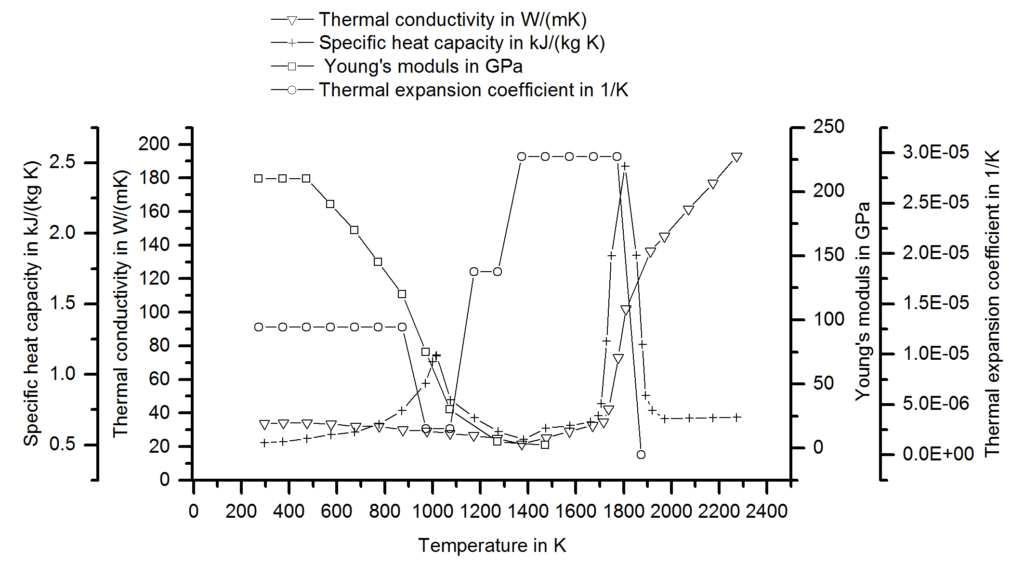
Figure 1: Material Data set for a DP1000.S-73
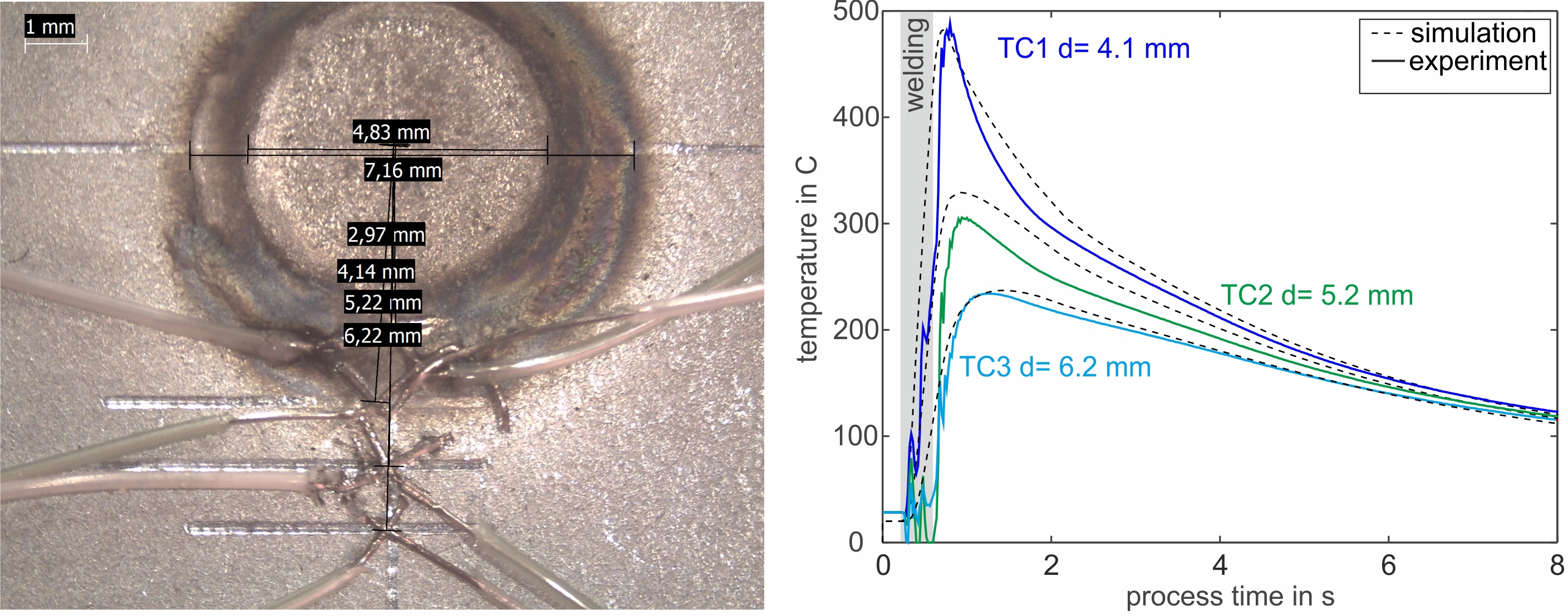
Next, meaningful boundary conditions must be chosen and validated against experiments. These include both the electrode cooling and the electrical contact resistance. To set up the thermal flow into the electrode, temperature measurements on the surface are common. In the following picture, a measurement with thermocouples during welding and the corresponding result is shown. By adjusting the thermal boundary in the model, the simulated temperatures are adjusted until a good match between simulation and experiment is visible. This calibration needs to be conducted only once when the model is established because the thermal boundary remains relatively constant for different materials and coatings.
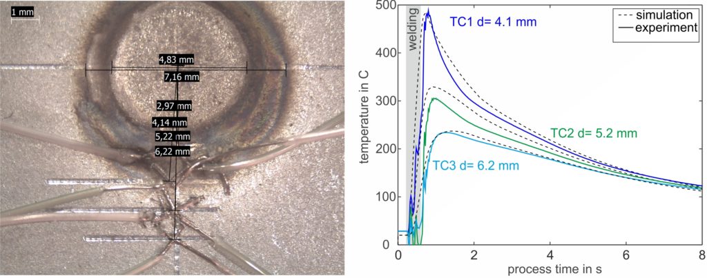
Figure 2: Temperature measurement with thermocouples during welding and the results. The simulated temperature development is compared to the experimental curve and can be adjusted via the boundary conditions.F-23
The second boundary condition is the electrical contact resistance and it is strongly dependent on the coating, the surface quality and the electrode force. It needs to be determined experimentally for every new coating and for as many material thickness combinations as possible. In the measuring protocol, a reference test eliminates the bulk material resistance and allows for the determination of the contact resistances using a µOhm-capable digital multimeter.
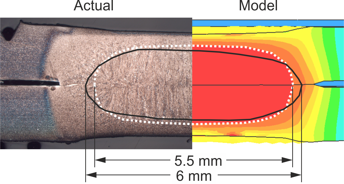
Finally, a metallographic cross-section shows whether the nugget size and -shape matches the experiment. The graphic shows a comparison between an actual and simulated cross section with a very small deviation of 0.5 mm in the diameter. As with the temperature measurements, a small deviation is not cause for concern. The experimental measurements also exhibit scatter, and there are a couple of simplifications in the model that will reduce the accuracy but still allow for fast calculation and good evaluation of trends.

Figure 3: Comparison of experimental and virtual cross-sections.F-23
After validation, consider conducting weldability investigations with the model. Try creating virtual force / current maps and the resulting nugget diameter to generate first guesses for experimental trials. We can also gain a feeling how the quality of each weld is affected by changes in coatings or by heated electrodes when we vary the boundary conditions for contact resistance and electrode cooling. The investigation of large spot-welded assemblies is possible for part fit-up and secondary effects such as shunting. Finally, the in-depth data on temperature flow and mechanical stresses is available for research-oriented investigations, cracking and joint strength impacts.
Note: The work represented in this article is a part a study of Liquid Metal Embrittlement (LME), commissioned by WorldAutoSteel. You can download the free report on the results of the LME study, including how this modelling was used to verify physical tests, from the WorldAutoSteel website.