Introduction Mechanical Joining Clinching Self-Pierce Riveting Flow Drill Screw Process Solid State Welding Ultrasonic Welding Friction Welding Diffusion Bonding Resistance Spot Welding Hybrid Welding Processes Introduction Multi material design approach is the...
Solid State Welding of Steel to Aluminum
read more