GMAW of Dissimilar AHSS Sheets

GMAW of Dissimilar AHSS Sheets

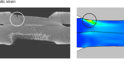
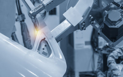
This is a summary of a paper of the same title, authored by K. Májlinger, E. Kalácska, and P. Russo Spena, used by permission.M-65


Researchers at the Budapest University of Technology and Economics and the Free University of Bozen-Bolzano tested gas metal arc welding (GMAW) of dissimilar Advanced High-Strength Steel (AHSS) sheets.M-65 The test pieces were 100 x 50 mm samples of 1.4 mm TWIP (TWIP1000) and 0.9 mm TRIP (HCTC800T) sheet steels were welded in a lap joint configuration with 0.8 mm diameter AWS ER307Si austenitic stainless steel wire to determine appropriate GMAW parameters for good quality welds. Quality was determined by external appearance, microstructure, and mechanical properties. Good welds were achieved with linear heat inputs (Q) with ranges from 500-650 kJ/m. The only fractures that occurred appeared within the weld bead by ductile failure modes. The HAZ of the TWIP steel showed grain coarsening and the HAZ of the TRIP steel experienced microstructural changes relative to the distance from the fusion boundary. The ultimate tensile strength (UTS) varies between 73%-84% of the weaker of the two steels.

Welding was conducted with an automated linear drive system with pure Argon (99.996% Ar) shielding gas at 10L/min. Wire feed rates were approximately 3.5 m/min with Direct Current Electrode Positive (DCEP) polarity. Changes in current, voltage, weld speed, and the resulting linear energy are compared in Table 1.

Figure 1: Overview of Dissimilar AHSS GMAW Welding.M-65

Figure 1: Overview of Dissimilar AHSS GMAW Welding.M-65


Table 1: Results of the preliminary welding tests in terms of TWIP-TRIP joint quality.M-65

Table 1: Results of the preliminary welding tests in terms of TWIP-TRIP joint quality.M-65


After welding, transverse sections were cut from the welds and etched to show the microstructure. Vickers hardness testing was conducted on the weld samples based on the ASTM E384 standard. Tensile tests were performed on the samples according to the EN ISO 6892-1 standard. Tests were also conducted on unwelded TWIP and TRIP steels for comparison. Scanning electron microscopy (SEM) examinations were made of fracture surfaces to determine failure modes and examine for microscopic weld defects.

The study concluded that dissimilar welds between AHSS steels with the GMAW process can be achieved with consistent results desired for automotive applications.

Figure 2: Vickers Hardness Across Weldment.M-65

Figure 2: Vickers Hardness Across Weldment.M-65


Figure 3: Ductile Failure in FZ.M-65

Figure 3: Ductile Failure in the fragile zones (FZ).M-65


Introduction

Introduction

The unique physical characteristics of Advanced High Strength Steels (AHSS) present some challenges to welding and bonding processes. AHSS differ from mild steels by chemical composition and microstructure, and it’s important to note that their microstructures will change from welding operations. For example, intensive localized heat associated with some welding processes causes a significant change in the local microstructure, and hence affect properties. Due to fast Cooling Rates (CR) typical in welding, it is normal to see martensite and/or bainite microstructures in the weld metal and in the Heat-Affected Zone (HAZ).

When joining AHSS, production process control is important for successful assembly. Manufacturers with highly developed joining control methodology will experience no major change in their operations. Others may require additional checks and maintenance. In certain instances, modifications to equipment or processing methodologies may be required for successful joining of AHSS.

The coating methods for AHSS are similar to those for mild steels. Welding of either AHSS or mild steels with coatings will generate fumes. The amount and nature of fumes will depend on the coating thickness, coating composition, joining method, and fillers used to join these materials. The fumes may contain some pollutants. The chemical composition of fumes and the relevant exhaust equipment must meet appropriate regulatory standards. Thicker coatings and higher heat inputs cause more fumes. Additional exhaust systems should be installed. While welding AHSS (with or without metallic or organic coatings and oiled or not oiled) gases and weld fumes are created similar to mild steels. The allowed fumes or gases must comply with respective national rules and regulations.

Joining Processes

Considering recent developments of hybrid approaches to welding, there are now over 100 types of welding processes available for the manufacturer or fabricator to choose from. The reason that there are so many processes is that each process has its list of advantages and disadvantages that make it more or less appropriate for a given application. Arc welding processes offer advantages such as portability and low cost but are relatively slow and use a considerable amount of heating to produce the weld. High energy density processes such as laser welding generally produce low heat inputs and fast welding speeds, but the equipment is very expensive and joint fit-up needs to be ideal. Solid-state welding processes avoid many of the weld discontinuities produced by those requiring melting (fusion), but they may be expensive and often are restricted to limited joint designs. Resistance welding processes are typically very fast and require no additional filler materials but are often limited to thin sheet applications or very high-production applications such as in the automotive industry.

Most welding processes produce a weld (metallic bond) using some combination of heat, time, and/or pressure. Those that rely on extreme heat at the source such as arc and high energy density processes generally need no pressure and relatively small-to-medium amounts of time. This section introduces joining processes that are applicable to HSS automotive applications, while describing unique process attributes.


LME Simulation During RSW

LME Simulation During RSW

Modern car bodies today are made of increasing volumes of Advanced High-Strength Steels (AHSS), the superb performance of which facilitates lightweighting concepts (see Figure 1). To join the different parts of a car body and create the crash structure, the components are usually welded to achieve a reliable connection. The most prominent welding process in automotive production is resistance spot welding. It is known for its great robustness, and easily applicable in fully automated production lines.

Figure 1: AHSS Content in Modern Car Body.W-7


There are, however, challenges to be met to guarantee a high-quality joint when the boundary conditions change, for example, when new material grades are introduced. Interaction of a liquefied zinc coating and a steel substrate can lead to small surface cracks during resistance spot welding of current AHSS, as shown in Figure 2. This so-called liquid metal embrittlement (LME) cracking is mainly governed by grain boundary penetration with zinc, and tensile stresses. The latter may be induced by various sources during the manufacturing process, especially under ‘rough’ industrial conditions. But currently, there is a lack of knowledge, regarding what is ‘rough’, and what conditions may still be tolerable.

Figure 2: Top View of LME-Afflicted Spot Weld.


The material-specific amount of tensile stresses necessary for LME enforcement can be determined by the experimental procedure ‘welding under external load’. The idea of this method, which is commonly used for comparing cracking susceptibilities of different materials to each other, is to apply increasing levels of tensile stresses to a sample during the welding process and monitor the reaction. Figure 3 shows the corresponding experimental setup.

Figure 3: Welding under external load setup.L-51


However, the known externally applied stresses are not exclusively responsible for LME, but also the welding process itself, which puts both thermally and mechanically induced stresses/strains on the sample. Here, the conventional measuring techniques fail. A numerical reproduction of the experiment grants access to the temperature, stress and strain fields present during the procedure, providing insights on the formation of LME. The electro-thermomechanical simulation model is described in detail in Modelling RSW of AHSS. It is used to simulate the welding under external load procedure (see Figure 4).

Figure 4: Simulation Model of Welding Under External Load.


The videos that can be found in the link above show the corresponding temperature and plastic strain fields. As heat dissipates quickly through the water-cooled electrode, a temperature gradient towards the adjacent areas and a local temperature maximum on the surface forms. The plastic strains accumulate mainly at the electrode indentation area. The simulated strain field shows a local maximum of plastic deformation at the left edge of the electrode indentation, amplified by the externally applied stresses and the boundary conditions implied by the procedure. This area correlates with experimentally observed LME cracking sites and paths as shown in Figure 5.

The simulation shows that significant plastic strains are present during welding. When external stresses (in reality e.g. due to poor part fit-up or distorted parts) contribute to the already high load, LME cracking becomes more likely. The numerical simulation model facilitates the determination of material-specific safety limits regarding LME cracking. Parameter variations and their effects on the LME susceptibility can easily be investigated by use of the model, enabling the user to develop strict processing protocols to reduce the likelihood of LME. Finally, these experimental procedures can be adapted to other high-strength materials, to aid their application understanding and industrial set-up conditions.

Figure 5: LME Cracks in Cross Section View at Highly Strained Locations.


For more information on this topic, see the paper, co-authored by Fraunhofer and LWF Paderborn, documented in Citation F-23.  You may also download the full report documenting the WorldAutoSteel LME project for which this work was conducted.


Dr.-Ing Max Biegler, Group Lead, Joining & Coating Technology
Fraunhofer Institute for Production Systems and Design Technology IPK
Modelling RSW of AHSS

Modelling RSW of AHSS

Modelling resistance spot welding can help to understand the process and drive innovation by asking the right questions and giving new viewpoints outside of limited experimental trials. The models can calculate industrial-scale automotive assemblies and allow visualization of the highly dynamic interplay between mechanical forces, electrical currents and thermal flow during welding. Applications of such models allow efficient weldability tests necessary for new material-thickness combinations, thus well-suited for applications involving Advanced High -Strength Steels (AHSS).

Virtual resistance spot weld tests can narrow down the parameter space and reduce the amount of experiments, material consumed as well as personnel- and machine- time. They can also highlight necessary process modifications, for example the greater electrode force required by AHSS, or the impact of hold times and nugget geometry. Other applications are the evaluation of whole-part distortion to ensure good part-clearance and the investigation of stress, strain and temperature as they occur during welding. This more research-focused application is useful to study phenomena arising around the weld such as the formation of unwanted phases or cracks.

Modern Finite-Element resistance spot welding models account for electric heating, mechanical forces and heat flow into the surrounding part and the electrodes. The video shows the simulated temperature in a cross-section for two 1.5 mm DP1000 sheets:


First, the electrodes close and then heat starts to form due to the electric current flow and agglomerates over time. The dark-red area around the sheet-sheet interface represents the molten zone, where the nugget forms after cooling. While the simulated temperature field looks plausible at first glance, the question is how to make sure that the model calculates the physically correct results. To ensure that the simulation is reliable, the user needs to understand how it works and needs to validate the simulation results against experimental tests. In this text, we will discuss which inputs and tests are needed for a basic resistance spot welding model.

At the base of the simulation stands an electro-thermomechanical resistance spot welding model. Today, there are several Finite Element software producers offering pre-made models that facilitate the input and interpretation of the data. First tests in a new software should be conducted with as many known variables as possible, i.e., a commonly used material, a weld with a lot of experimental data available etc.

As first input, a reliable material data set is required for all involved sheets. The data set must include thermal conductivity and capacity, mechanical properties like Young’s modulus, tensile strength, plastic flow behavior and the thermal expansion coefficient, as well as the electrical conductivity. As the material properties change drastically with temperature, temperature dependent data is necessary at least until 800°C. For more commonly used steels, high quality data sets are usually available in the literature or in software databases. For special materials, values for a different material of the same class can be scaled to the respective strength levels. In any case, a few tests should be conducted to make sure that the given material matches the data set. The next Figure shows an exemplary material data set for a DP1000. Most of the values were measured for a DP600 and scaled, but the changes for the thermal and electrical properties within a material class are usually small.

Figure 1: Material Data set for a DP1000

Figure 1: Material Data set for a DP1000.S-73

Next, meaningful boundary conditions must be chosen and validated against experiments. These include both the electrode cooling and the electrical contact resistance. To set up the thermal flow into the electrode, temperature measurements on the surface are common. In the following picture, a measurement with thermocouples during welding and the corresponding result is shown. By adjusting the thermal boundary in the model, the simulated temperatures are adjusted until a good match between simulation and experiment is visible. This calibration needs to be conducted only once when the model is established because the thermal boundary remains relatively constant for different materials and coatings.

Figure 2: Temperature measurement with thermocouples during welding and the results. The simulated temperature development is compared to the experimental curve and can be adjusted via the boundary conditions

Figure 2: Temperature measurement with thermocouples during welding and the results. The simulated temperature development is compared to the experimental curve and can be adjusted via the boundary conditions.F-23

The second boundary condition is the electrical contact resistance and it is strongly dependent on the coating, the surface quality and the electrode force. It needs to be determined experimentally for every new coating and for as many material thickness combinations as possible. In the measuring protocol, a reference test eliminates the bulk material resistance and allows for the determination of the contact resistances using a µOhm-capable digital multimeter.

Finally, a metallographic cross-section shows whether the nugget size and -shape matches the experiment. The graphic shows a comparison between an actual and simulated cross section with a very small deviation of 0.5 mm in the diameter. As with the temperature measurements, a small deviation is not cause for concern. The experimental measurements also exhibit scatter, and there are a couple of simplifications in the model that will reduce the accuracy but still allow for fast calculation and good evaluation of trends.

Figure 4: Comparison of experimental and virtual cross-sections.

Figure 3: Comparison of experimental and virtual cross-sections.F-23

After validation, consider conducting weldability investigations with the model. Try creating virtual force / current maps and the resulting nugget diameter to generate first guesses for experimental trials. We can also gain a feeling how the quality of each weld is affected by changes in coatings or by heated electrodes when we vary the boundary conditions for contact resistance and electrode cooling. The investigation of large spot-welded assemblies is possible for part fit-up and secondary effects such as shunting. Finally, the in-depth data on temperature flow and mechanical stresses is available for research-oriented investigations, cracking and joint strength impacts.

Note: The work represented in this article is a part a study of Liquid Metal Embrittlement (LME), commissioned by WorldAutoSteel.  You can download the free report on the results of the LME study, including how this modelling was used to verify physical tests, from the WorldAutoSteel website.

Dr.-Ing Max Biegler, Group Lead, Joining & Coating Technology
Fraunhofer Institute for Production Systems and Design Technology IPK


RSW Failure Prediction

RSW Failure Prediction

This article summarizes the findings of a paper entitled, “Prediction of Spot Weld Failure in Automotive Steels,”L-48 authored by J. H. Lim and J.W. Ha, POSCO, as presented at the 12th European LS-DYNA Conference, Koblenz, 2019.

To better predict car crashworthiness it is important to have an accurate prediction of spot weld failure. A new approach for prediction of resistance spot weld failure was proposed by POSCO researchers. This model considers the interaction of normal and bending components and calculating the stress by dividing the load by the area of plug fracture.


Background

Lee, et al.L-49 developed a model to predict spot welding failure under combined loading conditions using the following equation, based upon experimental results .

equation 1 Equation 1


Where FS and FN are shear and normal failure load, respectively, and n is a shape parameter.

Later, Wung and coworkersW-38 developed a model to predict the failure mode based upon the normal load, shear load, bending and torsion as shown in Equation 2.

equation 2 Equation 2


Here, FS, FN ,Mb and Mt are normal failure load, shear failure load, failure moment and failure torsion of spot weld, respectively.  α, β, γ and μ are shape parameters.

Seeger et al.S-106 proposed a model for failure criterion that describes a 3D polynomial failure surface. Spot weld failure occurs if the sum of the components of the normal, bending and shear stresses are above the surface, as shown in the Figure 1.

Figure 1. Spot weld failure model proposed by Seeger et al.S-106

Figure 1:  Spot weld failure model proposed by Seeger et al.S-106


The failure criterion can be expressed via Equation 3.

equation 3 Equation 3


Here, σN , σB , and τ are normal, bending and shear stress of the spot weld, respectively. And nN, nB and nc are the shape parameters. Toyota Motor CorporationL-50 has developed the stress-based failure model as shown in Equation 4.

equation 4 Equation 4


Hybrid Method to Determine Coefficients for Failure Models

This work used a unique hybrid method to determine the failure coefficients for modeling. The hybrid procedure steps are as follows:

  1. Failure tests are performed with respect to loading conditions.
  2. Finite element simulations are performed for each experiment.
  3. Based on the failure loads obtained in each test, the instant of onset of spot weld failure is determined. Failure loads are extracted comparing experiments with simulations.
  4. Post processing of those simulations gives the failure load components acting on spot welds such as normal, shear and bending loads.

These failure load components are plotted on the plane consisting of normal, shear and bending axes.

The hybrid method described above is shown in Figure 2.L-48

Figure 2:  Hybrid method to obtain the failure load with respect to test conditions.L-48

Figure 2:  Hybrid method to obtain the failure load with respect to test conditions.L-48


New Spot Weld Failure Model

The new proposed spot weld failure model in this paper considers only plug fracture mode as a normal spot weld failure. Secondly normal and bending components considered to be dependent upon each other. Stress generated by normal and bending components is shear, and shear component generates normal stress. Lastly authors have used πdt to calculate the area of stress instead of πd2/4. The final expression is shown in the Equation 5.

equation 5 Equation 5


Here τn is the shear stress by normal load components, σS is the normal stress due to shear load component. And , , c, α and β are coefficients.

This work included verification experiments of 42 kinds of homogenous steel stack-ups and 23 heterogeneous stack-ups. The strength levels of the steels used was between 270 MPa and 1500 MPa, and thickness between 0.55 mm and 2.3 mm. These experiments were used to evaluate the model and compare the results to the Wung model.

Conclusions

Overall, this new model considers interaction between normal and bending components as they have the same loading direction and plane. The current developed model was compared with the Wung model described above and has shown better results with a desirable error, especially for asymmetric material and thickness.


Microstructural Effects of Adding Colloidal Graphite to Al-Si-Coated PHS

Microstructural Effects of Adding Colloidal Graphite to Al-Si-Coated PHS

Optimizing weld morphology and mechanical properties of

laser welded Al-Si coated 22MnB5 by surface application of

colloidal graphite


Researchers at University of Waterloo discovered the microstructural effects of adding colloidal graphite to Al-Si coated 22MnB5 Press Hardened Steel.K-51 Laser welds were made on 1.5 mm thick Al-Si coated 22MnB5 PHS perpendicular to the rolling direction. Pure colloidal graphite suspended in isopropanol base was applied to the area being welded and the resulting graphite coating after evaporation ranged from 5 µm to 130 μm for testing. Parameters used for the weld are: 4kW power, 6m/min welding speed, beam diameter of 0.3 mm, and laser defocus of 6mm. Samples were then hot stamped by heating for 6 min to 930 ᵒC in a furnace and then water quenched at a cooling rate greater than 30 ᵒC/s.

Al-Si coating is excellent at preventing oxidation and decarburization of high strength steel at elevated temperatures. However, during welding there is diffusion of Al into the fusion zone which stabilizes ferrite at elevated temperature reducing the strength of the welded joint. Colloidal graphite coating decreases the Al content and increases C content of the fusion zone. As shown in Figure 1, The mechanism for reduction in Al content is due the graphite coating acting as an insulator to the Al-Si coating which then causes an ejection of the molten Al-Si coating from the surface. Figure 2 displays a proportional reduction of Al in the fusion zone with increasing graphite coating thickness up to 40 μm where after the reduction in Al is minimal. This is attributed to the initial reduction of Al being caused by the ejection of the molten Al-Si from underneath the graphite coating. Graphite coating greater than 40 µm does not aid in additional ejection of Al-Si and the Al-Si coating already diluted in the weld pool will not be removed.

Figure 1: Al-Si ejection mechanism.K-51

Figure 1: Al-Si ejection mechanism.K-51


Figure 2: Al and C content in weld with increasing graphite thickness

Figure 2: Al and C content in weld with increasing graphite thickness.K-51


Summary

Ferrite concentration in the fusion zone was reduced from approx. 40% with no graphite coating to approx. 2% with 130 μm graphite coating thickness (Figure 3). The increase in C content and reduction in Al content resulted in an increase in austenite being stabilized at elevated temperature rather than ferrite and therefore a larger percentage of martensite results after hot stamping. The average fusion zone hardness increased from 320 HV with no coating to 540 HV with 130 μm coating thickness (Figure 4). The weld strength of the sample with no graphite coating was 1249±15MPa whereas the weld strength with a coating of 130 µm was 1561±7MPa which matches the base metal (Figure 5). With an increase in graphite coating thickness there is an increase in weld strength that can eventually match the base metal strength.

Figure 3: Ferrite concentration in weld.K-51

Figure 3: Ferrite concentration in weld.K-51


Figure 4: Fusion Zone Hardness vs. Graphite Thickness.K-51

Figure 4: Fusion Zone Hardness vs. Graphite Thickness.K-51


Figure 5: Weld strength vs. Graphite Thickness.K-51

Figure 5: Weld strength vs. Graphite Thickness.K-51