The Need for Powertrain Models
Dr. Donald Malen, College of Engineering, University of Michigan, reviews the use of two recently developed Powertrain Models, which he co-authored with Dr. Roland Geyer, University of California, Bren School of Environmental Science.
The use of Advanced High-Strength Steel (AHSS) grades offer a means to lightweight a vehicle. Among the benefits of this lightweighting are less fuel used over the vehicle life, and better acceleration performance. Vehicle designers as well as Greenhouse Gas analysts are interested in estimating these benefits early in the vehicle design process. G-13
Models are constructed for this purpose which range from the use of a simple coefficient, (for example fuel consumption change per kg of mass reduction), to very detailed models accessible only to specialists which require knowledge of hundreds of vehicle parameters. Draw backs to the first approach is that the coefficient may be based on assumptions about the vehicle which do not match the current case. Drawbacks to the detailed models are the considerable expense and time needed, and the lack of transparency in the results; It is difficult to relate inputs with outputs.
A middle way between the simplistic coefficient and the complex model, is described here as a set of Parsimonious Powertrain Models. G-10, G-11, G-12 Parsimony is the principle that the best model is the one that requires the fewest assumptions while still providing adequate estimates. These Excel spreadsheet models cover Internal Combustion powertrains, Battery Electric Vehicles, and Plug-in Electric Vehicles, and predict fuel consumption and acceleration performance based on a small set of inputs. Inputs include vehicle characteristics (mass, drag coefficient, frontal area, rolling resistance), powertrain characteristics (fuel conversion efficiency, gear ratios, gear train efficiency), and fuel consumption driving cycle. Model outputs include estimates for fuel consumption, acceleration, and a visitation map.
Physics of the Models
Fuel consumption is determined by the quantity of fuel used over a driving cycle. The driving cycle specifies the vehicle speed vs. time. An example of a driving cycle is the World Light Vehicles Test Procedure (WLTP) cycle shown in Figure 1.
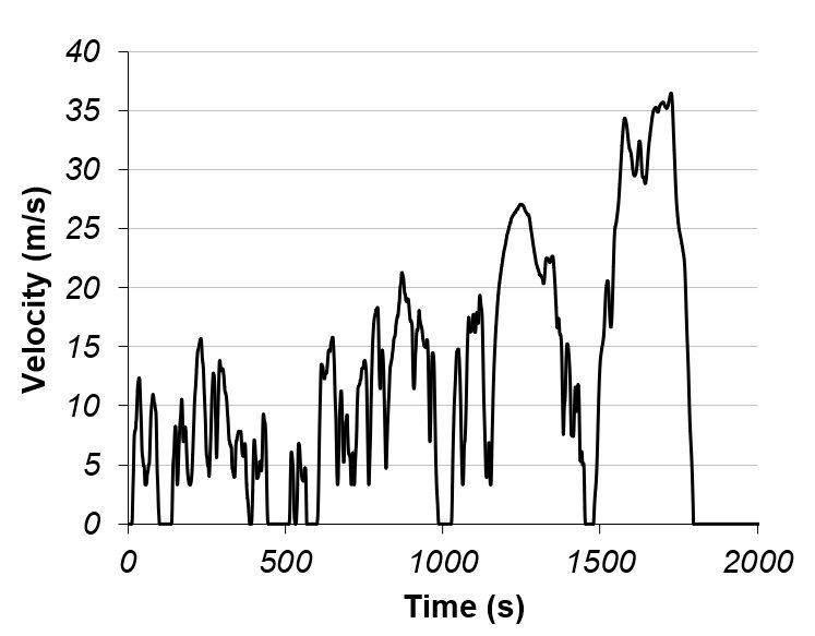
Figure 1: Fuel Consumption Driving Cycle (WLTP Class 3b).
Given the velocity history of Figure 1, the forces on the vehicle resisting forward motion may be calculated. These forces include inertia force, aerodynamic drag force, and rolling resistance. The total of these forces, called tractive force, must be provided by the vehicle propulsion system, see Figure 2.
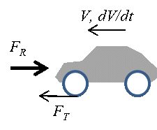
Figure 2. Tractive Force Required.
Once vehicle speed and tractive force are known at each point of time during the driving cycle, the required torque and rotational speed may be determined for each of the drivetrain elements, as shown in Figure 3 for an Internal Combustion system, and Figure 4 for a Battery Electric Vehicle.
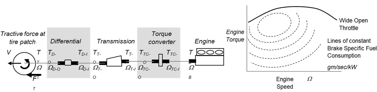
Figure 3. Internal Combustion Powertrain.
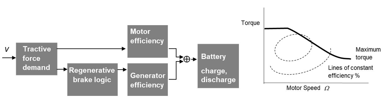
Figure 4. Battery Electric Vehicle Powertrain.
In this way, the required torque and speed of the engine or motor may be determined. Then using a map of efficiency, shown to the right in Figures 3 and 4, the energy demand is determined at each point in time. Summing the energy demand over time yields the fuel used over the driving cycle. The reader is referred to References 1 and 2 for a much more in depth description of the models.
Example Application
As an example application, consider the WorldAutoSteel FutureSteelVehicle (FSV).W-7 The FSV project, completed in 2011, investigated the weight reduction potential enabled with the use of AHSS, advanced manufacturing processes and computer optimization. The resulting material use in the body structure is shown in Figure 5.
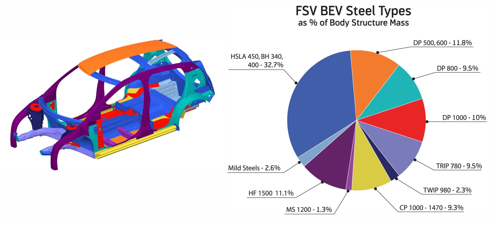
Figure 5. FutureSteelVehicle steel grade application.
This use of AHSS allowed a reduction in the vehicle curb mass from 1200 kg to 1000 kg. What are the effects of this mass reduction on fuel consumption and acceleration performance? The inputs required for the powertrain model are shown in Table 1 for the base case.
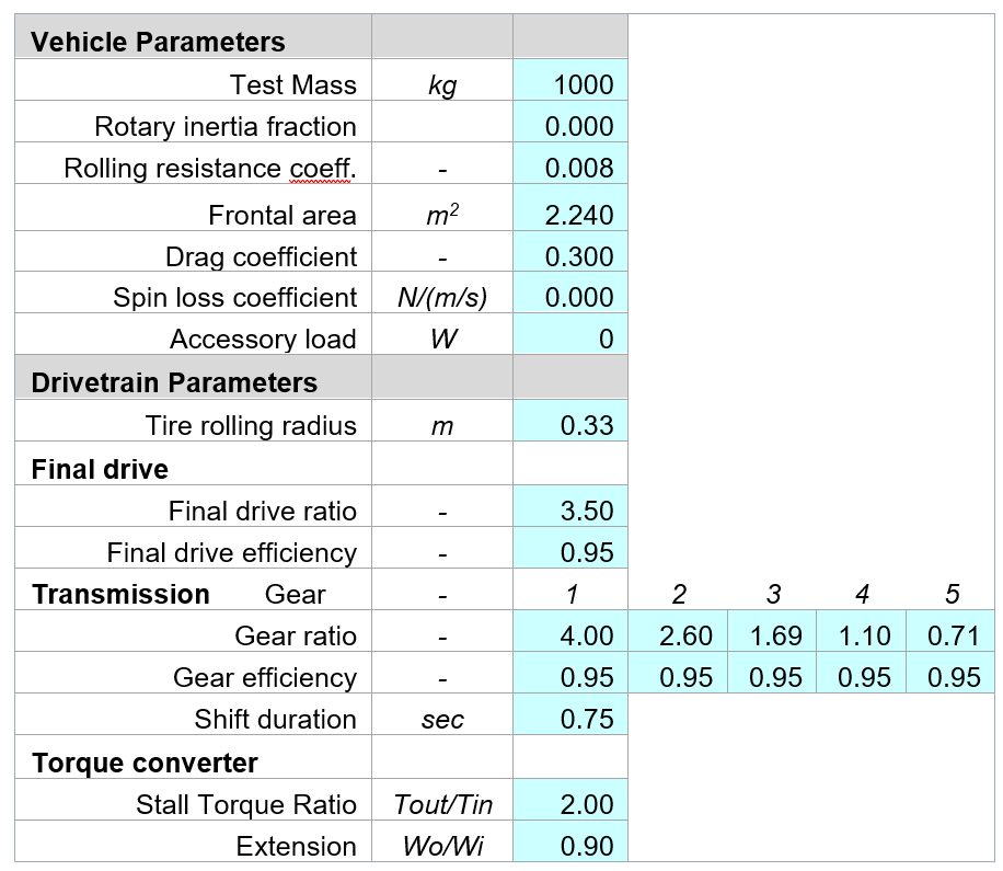
Table 1: Model Inputs for Base Case.
The results provided by the powertrain model are summarized in the acceleration-time vs. fuel consumption graph of Figure 6. Point A is the base case at 1200 kg curb mass. The lightweight case with same engine is shown as Point B. Note the fuel consumption reduction and also the acceleration time reduction. Often the acceleration time is set as a requirement. For the lighter vehicle, the engine size may be reduced to achieve the original acceleration time and an even greater reduction in fuel consumption as shown as Point C.
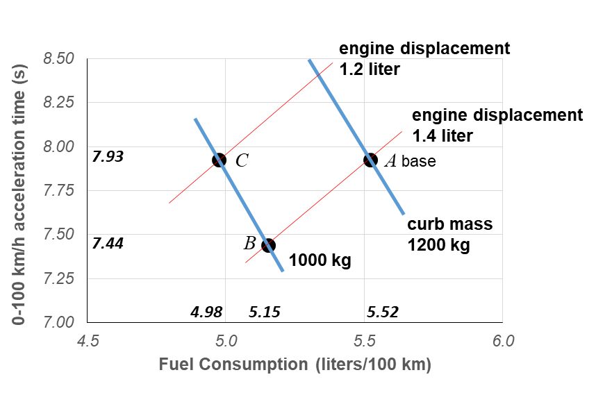
Figure 6. Summary of results of base vehicle and reduced mass vehicle.
Using the parsimonious powertrain models allows such ‘what-if’ questions to be answered quickly, with minimal data input, and in a transparent way. The Parsimonious Powertrain Models are available as a free download at worldautosteel.org.