As more companies aim to reduce their product’s time to market, research and design engineers have begun integrating predictive modeling into their process. These models, whether finite element based or artificial intelligence based, all rely on quality mechanical testing results. Companies within the automotive industry have seen that accurately predicting large scale tests such as crashworthiness trials can greatly expedite the time it takes to get their products to market. One of the more important details in predicting these expensive and time-consuming tests is to understand how the materials within the design are affected by the higher rates of deformation or their strain rates.
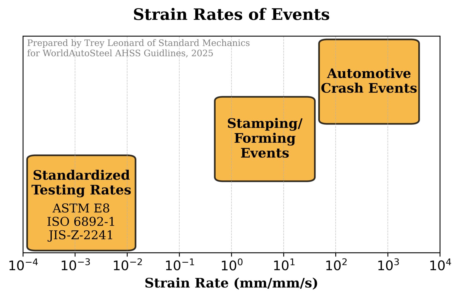
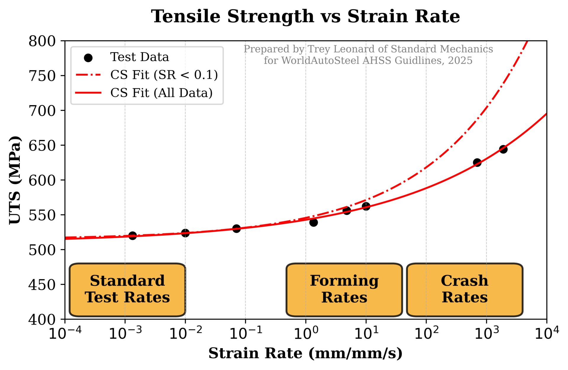
Traditional standardized tensile tests have been used for over a century – ASTM E8 was first approved in 1924. Testing laboratories using standards like ASTM E8, ISO 6892-1, and JIS Z-2241 produce repeatable and reproducible mechanical properties for metals undergoing tensile deformation, but each of these standards requires the test to be run at a speed orders of magnitude lower than those occurring during events like sheet metal forming and automotive crash. A tensile test run according to ASTM E8 to obtain the yield properties of a metal is run at a strain rate of 0.00035 strain per second (0.00035/s). For comparison, a stamping process has strain rates on the order of 1 to 10 strain per second, and an automotive crash can have strain rates up to 1,000 strain per second (Figure 1).
Figure 1. Strain rates of different events.
Historically, no guidelines have been available as to the testing method to obtain high strain rate mechanical properties. Decisions on specimen dimensions, measurement devices, and other important issues which are critical to the quality of testing results were made within each individual laboratory. As a result, data from different laboratories were often not directly comparable. A WorldAutoSteel committee evaluated various procedures, conducted several round-robins, and developed a recommended procedure, which evolved into what are now the first two parts of ISO 26203, linked below.
Published standards addressing tensile testing at high strain rates include:
Steel alloys typically possess positive strain rate sensitivity, or m-value when tested at ambient temperature, meaning that strength increases with strain rate. This has benefits related to improved crash energy absorption.
The specific response as a function of strain rate is grade dependent. Some grades get stronger and more ductile as the strain rate increases (left image in Figure 2), while other grades see primarily a strength increase (right image in Figure 2). Increases are not linear or consistent with strain rate, so simply scaling the response from conventional quasi-static testing does not work well. Strain hardening (n-value) also changes with speed in some grades, as suggested by the different slopes in the right image of Figure 2. Accurate crash models must also consider how strain rate sensitivity impacts bake hardenability and the magnitude of the TRIP effect, both of which are further complicated by the strain levels in the part from stamping.
Figure 2: Two steels with different strength/ductility response to increasing strain rate.A-7
Importance of Proper Testing Equipment
Knowing that the strain rate directly affects mechanical properties, many research test laboratories have run tensile tests using the same specimen geometry and machine as standardized but have increased the speed the machine runs during the test. This typically allows for tests to be performed at strain rates of up to 0.1 strain per second. From this data, an extrapolated curve can be fit to approximate the properties of the materials at higher strain rates. One model used to predict the increase in strength of a material deformed at a higher strain rate is the Cowper-Symonds model:
Equation 1
where σd is the strength of the material at a strain rate έ, σs is the strength of the material at a theoretical strain rate of zero strain per second, and C and p are model parameters.
Figure 3 shows two best fit curves for this Cowper-Symonds model to the tensile strengths of a cold rolled steel across a range of strain rates. The first considers only data that can be obtained using traditional tensile testing machines (strain rates less than 0.1 strain per second) while the second uses data up to 2,000 strain per second. Both models have minimal errors at strain rates below 0.1 strain per second, but as the limited model begins to extrapolate data beyond this strain rate regime, the associated error begins to grow exponentially causing large errors at the strain rates typical in crashes.
Figure 3. Example of extrapolation of tensile strength vs strain rate data using a Cowper-Symonds model. The dashed curve is an extrapolation based only on data acquired using traditional tensile testing machines, where strain rates are less than 0.1 strain per second. The solid curve is the extrapolation when considering data from equipment capable of achieving 2,000 strain per second.
Testing Methods and Equipment
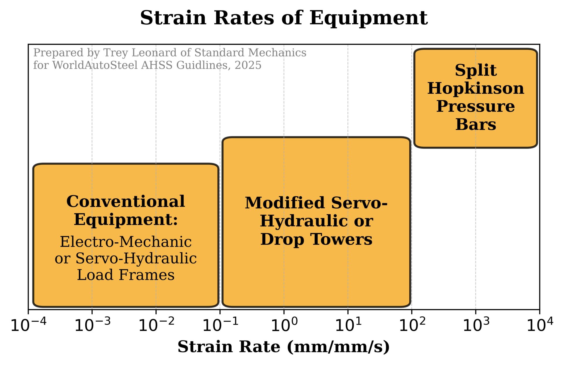
The biggest obstacle to measuring how a material responds to different strain rates is that it requires several different types of equipment. This is due to the need to run tests at up to six or seven different orders of magnitude to fully characterize the material. Figure 4 shows which mechanical testing equipment is most used to perform tensile tests based on the strain rate of the test. A broader range of testing methods for more strain rates can be found in the ASM Handbook, Volume 8: Mechanical Testing and Evaluation.A-88 The limits for the strain rate range that each type of test equipment can achieve varies based on the design and attributes of each specific machine as well as the specimen geometry used in testing. In tensile and compression testing, going from a longer specimen to a shorter specimen allows for a specific machine to increase its upper limit on strain rates.
Figure 4. Testing equipment most used to test materials at strain rates between 0.0001 strain per second and 10,000 strain per second in uniaxial tension.
Modified Servo-Hydraulic Machines
Modified servo-hydraulic testing machines are specifically engineered to characterize the dynamic mechanical properties of materials at high strain rates, often reaching strain rates up to 500 strain per second. Unlike conventional servo-hydraulic machines, which used closed-loop control for precise lower-speed testing, these modified systems incorporate design features that overcome the limitations of standard hydraulic controls at higher speeds. Many of these machines utilize extreme high flow valves along with slack adapters. The higher flow valves allow for higher accelerations while the slack adapters decouple the actuator from the specimen while the actuator accelerates to a desired test speed.
Split Hopkinson Pressure Bars
A split Hopkinson pressure bar (sometimes referred to as Kolsky bar or simply SHPB) is an impact-based device that is designed to characterize the dynamic mechanical properties of materials at strain rates above 100/s. The SHPB system uses a striker rod to generate a stress wave which induces plastic deformation in a specimen placed between two elastic bars. The stress wave generated by the striker bar in the first elastic bar (called the incident bar) is measured by a strain gauge fixed at the midpoint of the incident bar. When the stress wave reaches the specimen, part of the stress wave is transmitted through the specimen into the second elastic bar (called the transmitted bar) where it is measured by a second strain gauge. The rest of the stress wave is reflected off the specimen and returns down the incident bar to be re-measured by the strain gauge. Figure 5 shows how the stress waves propagate through a SHPB system during a compression test. There are various options to modify the compression SHPB setup to run a tensile test, but the most common is to replace the striker bar with a tube that slides on the incident bar where it impacts a flange on the end of the incident bar causing a tensile stress wave to propagate towards the specimen instead of a compression wave.
Figure 5. Animation showing how a stress wave propagates through a
split Hopkinson pressure bar system during a high strain rate compression test.
High Strain Rate Testing Challenges
Many other challenges complicate testing materials at higher strain rates. Three of the major challenges are
Challenges of measuring strain at high speeds
Challenges of accounting for inertial effects
Challenges of accounting for adiabatic heating
Strain Measurements in High Strain Rate Testing
During standardized mechanical testing, clip-on extensometers and deflectometers provide excellent extension measurements. As the speed of the test increases, the mass of the extensometer inhibits its use due to slippage of the contact points or interference with the specimen, both of which lead to erroneous test results and potential damage to the device. During high strain rate tests, the simplest means of measuring specimen displacements is to derive them based on the stress waves from the test. A detailed derivation of this method can be found here. This method works well for compression testing, but during tensile testing, events such as slippage of the specimen within the grips or deformation of the radius section of the specimen add to the displacements of the test. These additional displacements overshoot the tensile strain of a specimen during the test. This has led to the nearly universal adoption of optical strain measurements for high strain rate tension tests.
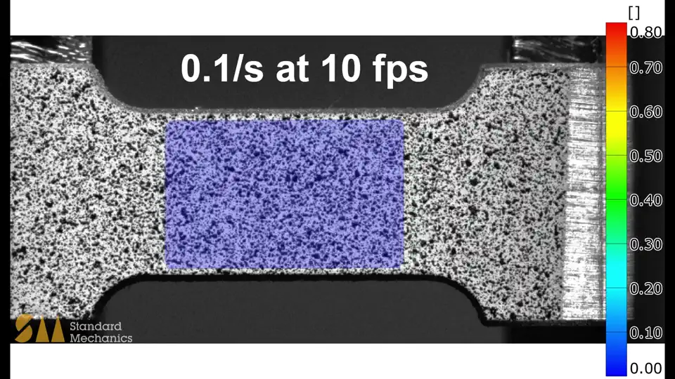
The most common optical method is digital image correlation (DIC). DIC correlates a series of images taken during the deformation of a specimen and calculates the corresponding strains of the specimen. It does this by tracking a black-and-white speckle pattern painted on the specimen’s surface which creates a series of high-contrast features as shown in Figure 6.
Figure 6. Two examples of 2D digital image correlation (DIC) showing the true equivalent strain fields during tensile tests performed at 0.1 strain per second and 1000 strain per second.
When testing round or more complex specimens, two cameras are required to track the surface of the specimen in three-dimensional space. This is referred to as 3D DIC, and it often requires more rigorous calibration for use in testing due to its multi-camera complexity. Alternatively, there are a series of one-dimensional options for strain measurements. The simplest utilizes a high-speed line scan camera to measure the displacement of a specimen along the test direction. While the two- and three-dimensional approaches bring in more data, the one-dimensional approach has been shown to provide excellent resolution at a lower adoption cost.Z-16
Accounting for Inertia in High Strain Rate Testing
At strain rates around one to ten strain per second, inertial effects can begin to complicate the interpretation of test results. These effects can be broken into two varieties: inertia of the specimen being tested and inertia of the equipment being used. Both directly affect the load values measured during a given test. In a modified servo-hydraulic load frame, large grips can create a large difference in stiffness (known more specifically as mechanical impedance) between each grip and the specimen. This difference causes more of any generated stress wave to be reflected at the interface as opposed to transmitting through; thus, as the wave travels back-and-forth through the specimen, the load it experiences “rings up”. This is sometimes referred to as “load ringing”. During this transient period of ring-up, the wave is amplifying or changing shape each time it reaches an end of the specimen. From this, the specimen experiences a load gradient across its gauge section depending on where the wave is at that point. After a certain number of reflections have occurred, the stress wave within the specimen becomes uniform and the specimen is determined to be in stress equilibrium. The number of oscillations it takes for this to occur is greatly dependent on the maximum frequency of the stress wave that enters the specimen and the ratio of mechanical impedances between the specimen and its grips. The lower the difference in impedances, the lower the energy that is reflected back into the specimen. The overall time of this period is not affected by the strain rate of the test being performed. This is because the phenomenon is based more so on the number of times the wave traverses the specimen which is solely dependent on the wave speed and length of the specimen. The wave speed of a material (assuming one—dimensional wave propagation) is calculated by:
Equation 2
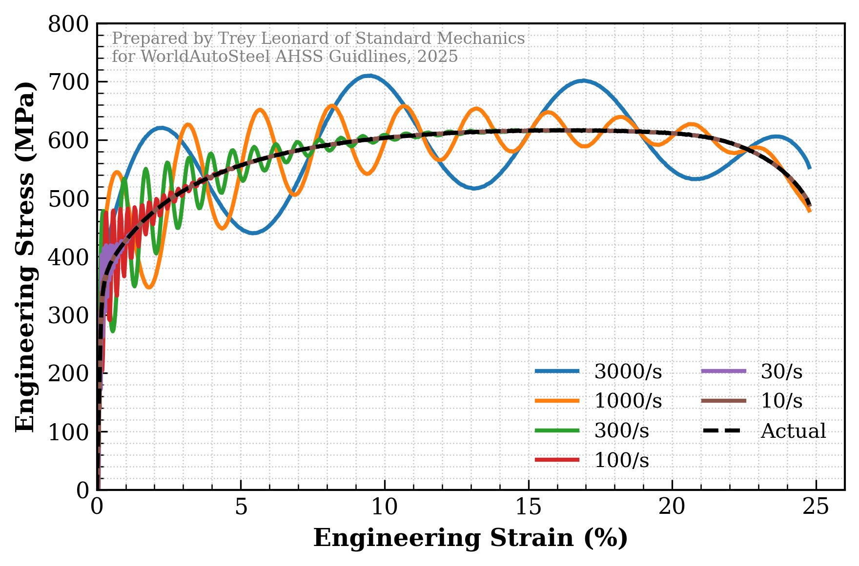
Where c is the wave speed of the material, E is the Young’s modulus of the material, and ρ is its density. When viewing test results, the load ringing can be seen as a decaying sinusoidal that begins when the specimen is first loaded. Figure 7 shows an example of how this could look across various strain rates. Each data set shares the same decay time constant, frequency, and magnitude of oscillations. Holding these three as constant simulates running tensile tests using the same specimen geometry, machine, and grips but varying the strain rate of the test. In the data set at lower strain rates, the effect of load ringing is minor with no notable difference between the actual response and the measured response at 10 strain per second. At 30 and 100 strain per second, the yield portions of the stress-strain curves are noisy, but the overall hardening profile is still clean. At 300 strain per second, the oscillations affect most of the hardening potion of the stress-strain curve. At 1000 strain per second, the overall profile of the stress-strain curve can be made out including strain to failure, but no details regarding hardening, uniform elongation, or tensile strength can be stated without large error bands. At 3000 strain per second, very little can be discerned from the data.
Figure 7. Illustration of theoretical frequency responses of dynamic tensile tests performed at various strain rates. All tests share the same decaying time constant, frequency, and magnitude of oscillations.
Some laboratories have adopted an inverse method that takes data with excessive load ringing and derives a stress-strain model. This is done by simulating the equipment used to perform the test along with the specimen tested in a finite element model. Then, repeated iterations of the stress-strain profile are sequentially optimized until the simulation best fits the data read from the test which includes the load oscillations. While this method has shown great potential, it is often too time intensive and expensive to justify in most industrial applications.
Adiabatic Heating in High Strain Rate Testing
The final challenge when testing materials at high strain rates comes from a by-product of plastic deformation of materials: adiabatic heating. Quasi-static tests allow for iso-thermal testing where the rate of heat being generated from plastically deforming the specimen is exceeded by the rate that heat is lost to the surrounding environment. As the strain rate of the test is increased, so too does the rate of plastic work and heat generation within the specimen. This internal heating is also compounded with the need for high intensity lighting to illuminate any high-speed optical methods for measuring strain of specimens. Because of these heat sources without equivalent cooling, the material response as measured by a high strain rate test is jointly affected by the higher strain rate as well as the elevated temperature of the specimen. These two effects have been shown experimentally to not be independent of one another, further complicating the analysis and interpretation of these tests. More complex multi-physics material models are often employed to account for these coupled effects in finite element model simulations.
Thanks are given to Trey Leonard, for his contributions to this page. Trey is the founder and CEO of Standard Mechanics, LLC, where he delivers advanced mechanical testing services and solutions across a wide range of applications, from automotive design to consumer electronics. His expertise spans formability, fatigue, and strain rate sensitivity testing. Beyond conducting tests, he partners with customers to ensure the development of high-quality, calibrated material cards and models for accurate finite element simulations. Dr. Leonard earned his Ph.D. in Mechanical Engineering from Mississippi State University, where he pioneered and licensed technologies in dynamic material testing and characterization. Building on this foundation, he continues to develop innovative testing methods and technologies that advance the field of dynamic mechanical testing. He also contributes to the broader engineering community through his work with ASTM International, where he serves on the E28 Committee on Mechanical Testing, regularly reviewing and improving industry standards.
Predicting metal flow and failure is the essence of sheet metal forming simulation. Characterizing the stress-strain response to metal flow requires a detailed understanding of when the sheet metal first starts to permanently deform (known as the yield criteria), how the metal strengthens with deformation (the hardening law), and the failure criteria (for example, the forming limit curve). Complicating matters is that each of these responses changes as three-dimensional metal flow occurs, and are functions of temperature and forming speed.
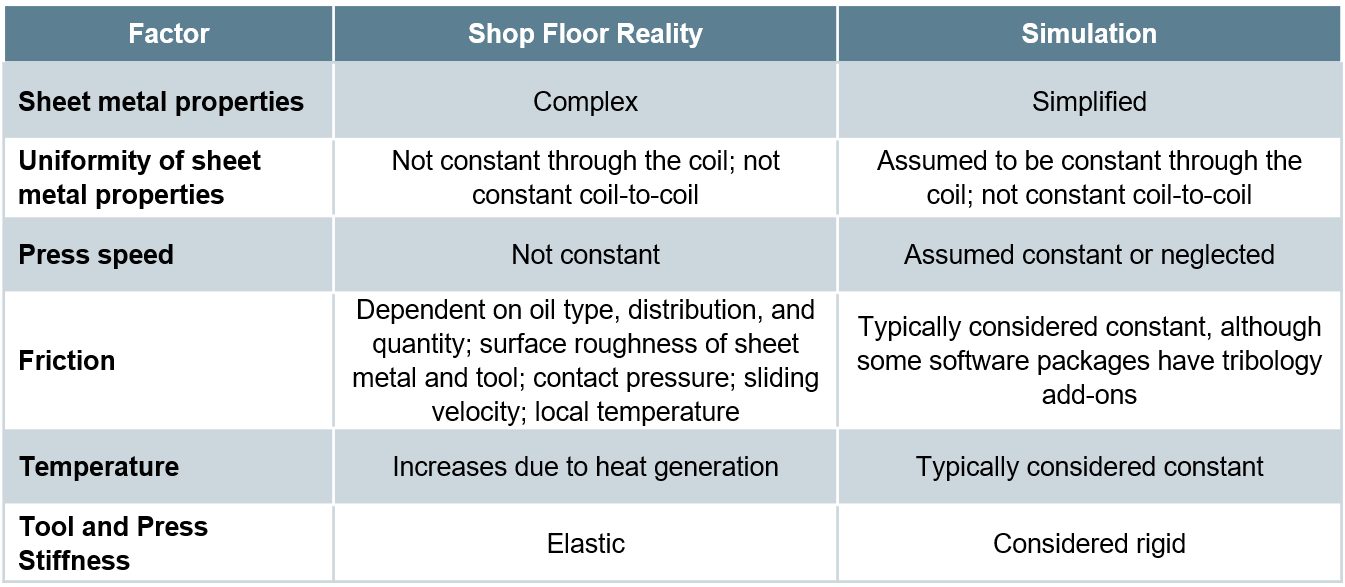
The ability to simulate these features reliably and accurately requires mathematical constitutive laws that are appropriate for the material and forming environments encountered. Advanced models typically improve prediction accuracy, at the cost of additional numerical computational time and the cost of experimental testing to determine the material constants. Minimizing these costs requires compromises, with some of these indicated in Table I created based on Citation R-28.
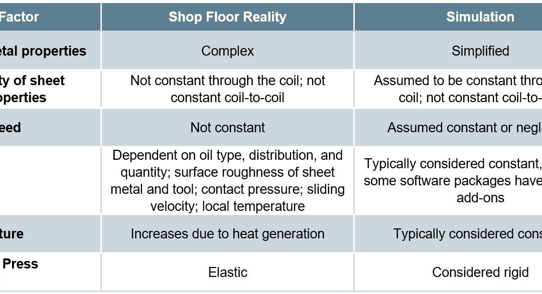
Table I: Deviations from reality made to reduce simulation costs. Based on Citation R-28.
Yield Criteria
The yield criteria (also known as the yield surface or yield loci) defines the conditions representing the transition from elastic to plastic deformation. Assuming uniform metal properties in all directions allows for the use of isotropic yield functions like von Mises or Tresca. A more realistic approach considers anisotropic metal flow behavior, requiring the use of more complex yield functions like those associated with Hill, Barlat, Banabic, or Vegter.
No one yield function is best suited to characterize all metals. Some yield functions have many required inputs. For example, “Barlat 2004-18p” has 18 separate parameters leading to improved modeling accuracy – but only when inserting the correct values. Using generic textbook values is easier, but negates the value of the chosen model. However, determining these variables typically is costly and time-consuming, and requires the use of specialized test equipment.
Hardening Curve
Metals get stronger as they deform, which leads to the term work hardening. The flow stress at any given amount of plastic strain combines the yield strength and the strengthening from work hardening. In its simplest form, the stress-strain curve from a uniaxial tensile test shows the work hardening of the chosen sheet metal. This approach ignores many of the realities occurring during forming of engineered parts, including bi-directional deformation.
Among the simpler descriptions of flow stress are those from Hollomon, Swift, and Ludvik. More complex hardening laws are associated with Voce and Hockett-Sherby.
The strain path followed by the sheet metal influences the hardening. Approaches taken in the Yoshida-Uemori (YU) and the Homogeneous Anisotropic Hardening (HAH) models extend these hardening laws to account for Bauschinger Effect deformations (the bending-unbending associated with travel over beads, radii, and draw walls).
As with the yield criteria, accuracy improves when accounting for three-dimensional metal flow, temperature, and forming speed, and using experimentally determined input parameters for the metal in question rather than generic textbook values.
Failure Conditions
Defining the failure conditions is the other significant challenge in metal forming simulation. Conventional Forming Limit Curves describe necking failure under certain forming modes, and are easier to understand and apply than alternatives. Complexity and accuracy increase when accounting for non-linear strain paths using stress-based Forming Limit Curves. Necking failure is not the only type of failure mode encountered. Conventional FLCs cannot predict fracture on tight radii and cut edges, nor can they account for dimensional issues like springback. For these, failure criteria definitions which are more mathematically complex are appropriate.
Constitutive Laws
Simple material models reduce the effort of testing, but may not be sufficiently accurate or do not apply to the spectrum of grades available today.
The yield surface constructed with Hill’48H-74 requires only data from three tensile tests. Models like Barlat-1989B-89, Barlet-2003B-90, Barlat-2005B-91, BBC2005B-92, VegterV-26, and Vegter liteV-27 all require data from more detailed advanced tests, but simulation results incorporating these yield surfaces more closely match experimental results.
Use caution with the assumptions that go into the Material Card. For example, the card may show the r-value in the rolling, diagonal, and transverse (0°, 45°, and 90°) orientations all the same (not realistic), or worse yet, all equal to 1. For high strength and advanced high strength steels, it is likely that at least one of the orientations will have an r-value below 1. In these cases assuming an r-value of 1 will lead to an underestimation of the thinning. Furthermore, use of the Hill 1948 yield criterion is not recommended since the model assumptions do not apply to r-values of less than 1.
The Keeler equation for FLC0K-71 requires only the n-value and thickness, but is based on a correlation established from grades and testing available no later than the early 1990s.
Predictive models for the yield surfaceA-96 and FLCsA-97 in cold stamping conditions were created to simplify the testing requirements while maintaining the accuracy and usefulness of these advanced models. These predictive equations have been validated against physical testing for mild steels, conventional high strength steels, advanced high strength steels, aluminum alloys, and stainless steel grades.
Similarly, for hot stamping, predictive models based on conventional tensile testing have been developed and verified.A-94, D-48, A-98 Challenges here include that elongation and r-value both vary with temperature and testing speed.
On the Forming Limit Curve shown in Figure 1a, the uniaxial strain path, plane strain, biaxial, and balanced biaxial points are predicted from total elongation (A80) and r-value determined from tensile testing in the 0, 45 and 90° orientations with respect to rolling direction.A-94 Compared with the Keeler model, the Abspoel & Scholting model is better at predicting the FLC of DP800, noting the upper limiting strains found in the experiment match the FLC, as well as a more accurate representation of the slope on the LH side. Both models appear sufficient for the conventional grade DC04 (similar to CR3).
Figure 1. a) FLC prediction locations. b) FLC comparison on drawing steel DC04 (CR3); c) FLC comparison on DP800.A-94
Yield surface correlations use Tensile strength (Rm), uniform elongation (Ag) and r-value test data as inputs to predict the equi-biaxial, plane strain and shear points in three directions. Figure 2 compares biaxial yield strength predictions between Hill’48 and Vegter 2017, showing the improved correlation in the model developed almost 70 years later.
Figure 2. Comparison of measured biaxial yield strength with prediction from Hill’48 (red) and Vegter 2017 (yellow).A-94
Figure 3 presents a comparison of the measured yield surfaces of DX54D+Z (galvanized CR3) and DP1000 with those predicted by Hill’48 and Vegter 2017, highlighting the improved accuracy found in Vegter 2017.
Figure 3. Comparison of measured yield surface with predictions from Hill’48 and Vegter 2017. a) DX54D+Z (galvanized CR3); b) DP1000.A-94
Material properties like elongation, r-value, the hardening curve, and forming limits are all likely both strain-rate and temperature dependent, meaning that a rate-dependent and temperature-dependent yield surface and forming limit curve are needed for more accurate representations of cold- and hot-stamping.
The initial implementation of the Vegter yield surface in forming simulation software packages showed satisfactory correlation with conventional stamping applications, but was sub-optimal in operations where stresses are found in the thickness direction such as coining, wall ironing and score forming processes in packaging and battery applications. In these cases, a non-convexity close to the equi-biaxial point of the yield locus was observed, likely due to extreme anisotropy or very low r-values.
Citation A-95 discusses methods for improved accuracy. DIC measurements offer improved r-value characterization over mechanical measurement approaches. Yield locus correlations at low and high plastic strain ratios were also improved. Shell elements used in the simulation of the yield surface in plane stress ignore the strains in the through-thickness direction. For the applications where thickness stresses play a role (like wall ironing, coining, score forming in packaging, and sharp radii in closures, solid or thick shell elements are required. The yield surface was extended to the thickness direction to allow for improved characterization in these applications having significant stresses through the thickness. This extension may be deployed in forming simulation software as “Vegter 2017.1.”
Constitutive Laws and Their Influence on Forming Simulation Accuracy
Many simulation packages allow for an easy selection of constitutive laws, typically through a drop-down menu listing all the built-in choices. This ease potentially translates into applying inappropriate selections unless the simulation analyst has a fundamental understanding of the options, the inputs, and the data generation procedures.
Some examples:
The “Keeler Equation” for the estimation of FLC0has many decades of evidence in being sufficiently accurate when applied to mild steels and conventional high strength steels. The simple inputs of n-value and thickness make this approach particularly attractive. However, there is ample evidence that using this approach with most advanced high strength steels cannot yield a satisfactory representation of the Forming Limit Curve.
Even in cases where it is appropriate to use the Keeler Equation, a key input is the n-value or the strain hardening exponent. This value is calculated as the slope of the (natural logarithm of the true stress):(natural logarithm of the true strain curve). The strain range over which this calculation is made influences the generated n-value, which in turn impacts the calculated value for FLC0.
The strain history as measured by the strain path at each locationgreatly influences the Forming Limit. However, this concept has not gained widespread understanding and use by simulation analysts.
A common method to experimentally determine flow curves combines tensile testing results through uniform elongation with higher strain data obtained from biaxial bulge testing. Figure 4 shows a flow curve obtained in this manner for a bake hardenable steel with 220 MPa minimum yield strength. Shown in Figure 5 is a comparison of the stress-strain response from multiple hardening laws associated with this data, all generated from the same fitting strain range between yield and tensile strength. Data diverges after uniform elongation, leading to vastly different predictions. Note that the differences between models change depending on the metal grade and the input data, so it is not possible to say that one hardening law will always be more accurate than others.
Figure 4: Flow curves for a bake hardenable steel generated by combining tensile testing with bulge testing.L-20
Figure 5: The chosen hardening law leads to vastly different predictions of stress-strain responses.L-20
Analysts often treat Poisson’s Ratio and the Elastic Modulus as constants. It is well known that the Bauschinger Effect leads to changes in the Elastic Modulus, and therefore impacts springback. However, there are also significant effects in both Poisson’s Ratio (Figure 6) and the Elastic Modulus (Figure 7) as a function of orientation relative to the rolling direction. Complicating matters is that this effect changes based on the selected metal grade.
Figure 6: Poisson’s Ratio as a Function of Orientation for Several Grades (Drawing Steel, DP 590, DP 980, DP 1180, and MS 1700) D-11
Figure 7: Modulus of Elasticity as a Function of Orientation for Several Grades (Drawing Steel, DP 590, DP 980, DP 1180, and MS 1700) D-11
Testing to Determine Inputs for Simulation
Complete material card development requires results from many tests, each attempting to replicate one or more aspects of metal flow and failure. Certain models require data from only some of these tests, and no one model typically is best for all metals and forming conditions. Tests described below include:
Tensile testing [room temperature at slow strain rates to elevated temperature with accelerated strain rates]
Biaxial bulge testing
Biaxial tensile testing
Shear testing
V-bending testing
Tension-compression testing with cyclic loading
Friction
Tensile testing is the easiest and most widely available mechanical property evaluation required to generate useful data for metal forming simulation. However, a tensile test provides a complete characterization of material flow only when the engineered part looks like a dogbone and all deformation resulted from pulling the sample in tension from the ends. That is obviously not realistic. Getting tensile test results in more than just the rolling direction helps, but generating those still involves pulling the sample in tension. Three-dimensional metal flow occurs, and the stress-strain response of the sheet metal changes accordingly.
The uniaxial tensile test generates a draw deformation strain state since the edges are free to contract. A plane strain tensile test requires using a modified sample geometry with an increased width and decreased gauge length,
Forming all steels involves a thermal component, either resulting from friction and deformation during “room temperature” forming or the intentional addition of heat such as used in press hardening. In either case, modeling the response to temperature requires data from tests occurring at the temperature of interest, at appropriate forming speeds. Thermo-mechanical simulators like Gleeble™ generate such data.
Conventional tensile testing occurs at deformation rates of 0.001/sec. Most production stamping occurs at 10,000x that amount, or 10/sec. Crash events can be 2 orders of magnitude faster, at about 1000/sec. The stress-strain response varies by both testing speed and grade. Therefore, accurate simulation models require data from higher-speed tensile testing. Typically, generating high speed tensile data involves drop towers or Split Hopkinson Pressure Bars.
A pure uniaxial stress state exists in a tensile test only until reaching uniform elongation and the beginning of necking. Extrapolating uniaxial tensile data beyond uniform elongation risks introducing inaccuracies in metal flow simulations. Biaxial bulge testing generates the data for yield curve extrapolation beyond uniform elongation. This stretch-forming process deforms the sheet sample into a dome shape using hydraulic pressure, typically exerted by water-based fluids. Citation I-12describes a standard test procedure for biaxial bulge testing.
A Marciniak test used to create Forming Limit Curves generates in-plane biaxial strains. Whereas FLC generation uses 100 mm diameter samples, larger samples allow for extraction of full-size tensile bars. Although this approach generates samples containing biaxial strains, the extracted samples are tested uniaxially in the conventional manner.
Biaxial tensile testing allows for the determination of the yield locus and the biaxial anisotropy coefficient, which describes the slope of the yield surface at the equi-biaxial stress state. This test uses cruciform-shaped test pieces with parallel slits cut into each arm. Citation I-13 describes a standard test procedure for biaxial tensile testing. The biaxial anisotropy coefficient can also be determined using the disk compression testing as described in Citation T-21.
Shear testing characterizes the sheet metal in a shear loading condition. There is no consensus on the specimen type or testing method. However, the chosen testing set-up should avoid necking, buckling, and any influence of friction.
V-bending testsdetermine the strain to fracture under specific loading conditions. Achieving plane strain or plane stress loading requires use of a test sample with features promoting the targeted strain state.
Tension-compression testing characterizes the Bauschinger Effect. Multiple cycles of tension-compression loading captures cyclic hardening behavior and elastic modulus decay, both of which improve the accuracy of springback predictions.
The Bauschinger effect leads to early re-yielding after loading reversal, and has been observed in loading-reverse loading testing. The Yoshida-Uemori (YU) kinematic hardening model accurately captures the Bauschinger effect as well as other hardening behaviors of sheet metals during loading-reverse loading.Y-7, Y-8
Characteristics of the Bauschinger Effect (Figure 8) include a) the transient Bauschinger deformation characterized by early re-yielding and smooth elastic–plastic transition with a rapid change of the work hardening rate; b) the permanent softening characterized by a stress offset observed in a region after the transient period; and c) work-hardening stagnation appearing at a certain range of reverse deformation.Y-7
Figure 8: Characteristics of the Bauschinger Effect during cyclic loading.Y-7
Citation L-78 describes an approach to calibrate the YU model on a QP1500 steel that uses a combination of physical testing and machine learning to achieve loading-reverse loading stress-strain curves over broader strain ranges. This citation also reported that the results from tension-compression testing were not the same as those from compression-tension testing – meaning that the order of deformation influences the results.
However, no standard procedure exists for determining the kinematic hardening and Bauschinger parameters and subsequently incorporating it into metal forming simulation codes. Independent of the procedure, one of the biggest challenges with this test is preventing buckling from occurring during in-plane compressive loading. Related to this is the need to compensate for the friction caused by the anti-buckling mechanism in the stress-strain curves.
Frictionis obviously a key factor in how metal flows. However, there is no one simple value of friction that applies to all surfaces, lubricants, and tooling profiles. The coefficient of friction not only varies from point to point on each stamping but changes during the forming process. Determining the coefficient of friction experimentally is a function of the testing approach used. The method by which analysts incorporate friction into simulations influences the accuracy and applicability of the results of the generated model.
Studies are underway to reduce the costs and challenges of obtaining much of this data. It may be possible, for example, to use Digital Image Correlation (DIC) during a simple uniaxial tensile testing to quantify r-value at high strains, determine the material hardening behavior along with strain rate sensitivity, assess the degradation of Young’s Modulus during unloading, and use the detection of the onset of local neck to help account for non-linear strain path effects.S-110
Application of Advanced Testing to Failure Predictions
Global formability failures occur when the forming strains exceed the necking forming limit throughout the entire thickness of the sheet. Advanced steels are at risk of local formability failures where the forming strains exceed the fracture forming limit at any portion of the thickness of the sheet.
Fracture forming limit curves plot higher than the conventional necking forming limit curves on a graph showing major strain on the vertical axis and minor strain on the horizontal axis. In conventional steels the gap between the fracture FLC and necking FLC is relatively large, so the part failure is almost always necking. The forming strains are not high enough to reach the fracture FLC.
In contrast, AHSS grades are characterized by a smaller gap between the necking FLC and the fracture FLC. Depending on the forming history, part geometry (tight radii), and blank processing (cut edge quality), forming strains may exceed the fracture FLC at an edge or bend before exceeding the necking FLC through-thickness. In this scenario, the part will fracture without signs of localized necking.
This collection of studies, as well as work coming out of these studies, show that relatively few tests sufficiently characterize forming and fracture of AHSS grades. These studies considered two 3rd Gen Steels, one with 980MPa tensile strength and one with 1180MPa tensile.
The yield surface as generated with the Barlat YLD2000-2d yield surface (Figure 9) comes from:
Conventional tensile testing at 0, 22.5, 45, 67.5, and 90 degrees to the rolling direction, determining the yield strength and the r-value;
Disc compression tests according to the procedure in Citation T-21 to determine the biaxial R-value, rb.
Figure 9: Tensile testing and disc compression testing generate the Barlat YLD2000-2d yield surface in two 3rd Generation AHSS Grades B-13
Creating the hardening curve uses a procedure detailed in Citations R-5 and N-13, and involves only conventional tensile and shear testing using the procedure included in Citation P-15.
Figure 10: Test geometries for hardening curve generation. Left image: Tensile; Right image: Shear.N-13
Characterizing formability involved generating a Forming Limit Curve using Marciniak data or process-corrected Nakazima data. (See our article on non-linear strain paths) and Citation N-13 for explanation of process corrections]. Either approach resulted in acceptable characterizations.
Fracture characterization uses four plane stress tests: shear, conical hole expansion, V-bending, and a biaxial dome test. The result from these tests calibrate the fracture locus describing the stress states at fracture.
A different approach requires only the results from conventional tensile testing and a crack growth test under simple loading to simulate post-necking strain hardening behavior and ductile fracture. The details of this approach are beyond the scope of this webpage, but are presented in detail in Citations S-124 and T-56, in addition to verification procedures.
Simulation Set-Up Parameters
One of the most basic choices when starting a simulation run is the setting related to the mesh size. Reduced processing time is associated with large mesh sizes, but that risks not having sufficiently fine mesh resolution to capture the forming strain gradient. A large mesh size averages the strains over a larger region, which is analogous to a tensile bar with an 80 mm gauge length having lower elongation than a 50 mm tensile bar cut from the same sheet steel.
Figure 11 compares the Forming Limit Curve (FLC) for an 1180 MPa steel determined from gauge lengths of 2, 6, and 10 mm, along with the associated theoretical predictions. As expected, the smaller gauge length is able to more effectively capture peak strains, and is therefore associated with a higher forming limit.A-90
Figure 11: Comparison of predicted values and experimental values of the Forming Limit Curve of an 1180 MPa steel.A-90
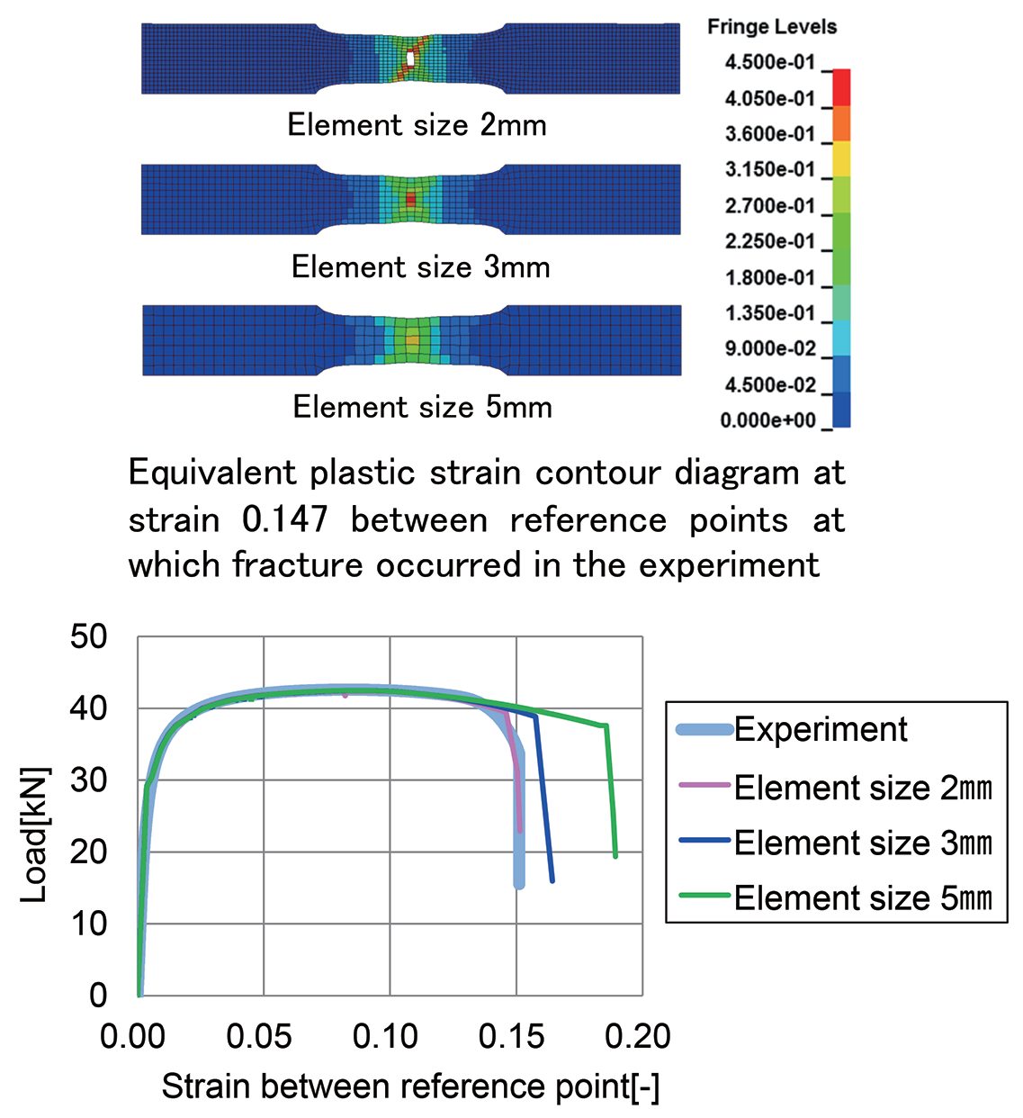
The stress-strain curve of a 1.6 mm 980 MPa steel tested with a 50 mm gauge length (ISO III, JIS) was captured, resulting in a strain at fracture of 0.147. A model based on a 2 mm element size was created, calibrated to the same strain at fracture of 0.147. The model was re-run with element sizes of 3 mm and 5 mm, which resulted in different stress strain curves and simulations that could not predict the fracture known to occur, Figure 12. This study also showed a technique that can be used to achieve similar performance nearly independent of mesh size, such that accuracy is not compromised when optimizing computer processing speed.A-90
Figure 12: Comparison of the tensile test result and fracture model predictions based on different element sizes.A-90
Constitutive Models
Constitutive models for steel strengthening fall into two general categories: power law behavior like HollomonH-71 and SwiftS-119 or saturation models like Voce and Hockett-Sherby.H-72 As shown in Figure 2 above, the chosen constitutive model significantly influences the extrapolation of experimental stress-strain curves to larger strain values. Model combinations such as Swift-Voce or Swift/Hockett-Sherby, typically using one for lower strains and the other for higher strains, typically provide better fit with experimental dataK-65, but more parameters are usually beneficial, especially for advanced high strength steels where the n-value is not constant with strain.
To improve the modeling accuracy of high strength steels with variable instantaneous n–value, hardening curves obtained with uniaxial tensile and hydraulic bulge tests were fit to a new proposed modelL-73 to verify its predictive capability and accuracy. This new model, based on the Swift power law (Equation 1), addresses the decrease in n-value at larger plastic strains by varying what has been termed as the strain hardening attenuation coefficient a, within a new parameter λh as defined in Equation 2.
Equation 1
Equation 2
When a=0, Equation 1 reverts to the standard Swift equation. When a>0, it allows for Equation 1 to correct for the decrease of instantaneous n value occurring at larger plastic strains. The results in Figure 133 show that the predictive accuracy of the new model is better than the individual Swift or Hockett-Sherby models.
Figure 13: Hardening Curve for two grades showing Uniaxial Tensile (ut) stress-strain curves, biaxial tensile extension from biaxial bulge testing (bt), Swift and Hockett-Sherby model fit, and new model fit with different a parameter.L-73
Experimental hardening data for a QP grade, referred to as QP1180-EL, was obtained from uniaxial tensile testing combined with bulge testing and in-plane torsion testing for strains beyond uniform elongation. These are shown as squares and black or red circles in Figure 14, along with projections from the Swift and Hockett-Sherby models. The Modified Power Law (MPL) achieves the best fit to the tested results.Z-18
Figure 14: Experimental results compared with the Swift power law hardening model, Hockett-Sherby saturation hardening model, and a newly developed Modified Power Law.Z-18
Improved vehicle crashworthiness predictions occur when the forming history of the critical structural parts, including the effects of bake hardening, work hardening, and thickness reduction, are incorporated into vehicle virtual development models. Historically, simulations did not contemplate the initial damage caused by plastic deformation. Accumulated damage can be captured within a GISSMO (Generalized Incremental Stress State Dependent Model) damage model, albeit with certain assumptions.N-30, N-31
Five different loading cases capturing the stress state of shear, uniaxial tension, stretching, plane strain and equi-biaxial stretching can be used to calibrate parameters of the Modified Mohr-Coulomb (MMC) B-83 fracture model. Schematics of these five individual tests are shown in Figure 15.H-73 The calibrated MMC model and loading path results from these tests are shown in Figure 16. The MMC model was subsequently used to calibrate a GISSMO damage model.
Figure 15: Tests coupons for fracture model calibration.H-73
Figure 16. Calibrated MMC fracture model and loading path results from the tests shown in Figure 10.H-73
Quasi-static three-point quasi-static bending tests were used to validate the MPL hardening model, the MMC fracture model, and the GISSMO damage model. An FEA model with a 2 mm mesh size was compared with one having a 5 mm mesh size for the simulation of the bending process. Figure 17 shows the predicted fracture location and test result.
Local necking was observed during the experimental bending test and 2 elements failed in when using a 2 mm mesh size, yet no failure was observed when using a 5 mm mesh. This indicates that accurate simulation results may require refined mesh sizes.
Figure 17: Experiment and simulation results of three-point bending testing of a Quenched & Partitioned 1180 MPa Steel.H-73
A subsequent studyZ-18 confirmed that ignoring the stamping forming history in the damage model results in a lower prediction of the failure risk, especially for cold stamping high-strength steel parts under large deformation conditions.
Case Studies: Benefits of using Advanced Models for Springback Prediction
The output of simulations using material models that thoroughly capture the changes in metal properties occurring during forming are more likely to match reality than those simulations based on basic models.
Kinematic hardening models where the Bauschinger effect and modulus degradation are captured have been shown to be substantially more accurate in springback prediction than isotropic hardening models based on more conventional tensile testing.
Citation S-130 investigated this difference. Different types of steels having 980 MPa or 1180 MPa minimum specified tensile strength from multiple suppliers were used to form a targeted part shape using either a draw forming process or a crash forming process. The formed panels were scanned and compared with simulation results from multiple software packages. In all cases, the simulation was capable of accurately predicting strains and the risk of necking failure.
For springback, the type of hardening model used in the simulation appeared to correlate with prediction ability. Table 2 compares the dimensional difference between the model and a scan of the physical panel, with smaller numbers representing an improved ability to predict springback in the evaluated condition. As indicated in Table 2, models incorporating Kinematic Hardening more closely matched the actual springback seen on the scanned panels.
Table 2: Dimensional Deviation Between Simulation and Scan as a Function of Hardening Model.S-130
Maximum Sectional Deviation
During Draw Forming (mm)
Maximum Sectional Deviation
During Crash Forming (mm)
Hardening Model
5.38
5.54
Isotropic Hardening
5.25
2.27
Yoshida
5.01
10.2
Isotropic Hardening
4.2
2.422
Hill ’48 Isotropic Hardening
4.17
3.127
Hill ’48 Isotropic Hardening
3.14
2.8
Yoshida
3.12
5.3
Yoshida
2.65
N/A
Yoshida
2.3
4.2
Yoshida-Uemori
2.17
7.39
Yoshida
1.98
1.64
Yoshida-Uemori
1.797
1.952
Yoshida
1.5
2.3
Yoshida
Results compiled across multiple types of simulation software,
compared with formed parts made from different types of 980 and 1180 grades from multiple suppliers.
A modified S-shape generic panel was used to evaluate springback using a 3rd Generation Steel having a minimum specified tensile strength of 980MPa.B-98 Nearly 200 points were evaluated on the panel shown in Figure 18. For the simulation that did not incorporate kinematic hardening, 48% of this panel were within 1 mm of the physical scanned part and 32% were within 0.5 mm. When the simulation incorporated kinematic hardening, 94% of the points were within 1 mm and 60% were within 0.5 mm.
Figure 18: Modified S-Shape used to evaluate springback on 3rd Gen 980 MPa steel in Citation B-98.
A generic B-pillar panel was used to evaluate springback using a 3rd Generation Steel having a minimum specified tensile strength of 1180MPa.K-72
For the simulation that did not incorporate kinematic hardening, 59.9% of this panel were within 1 mm of the physical scanned part. When the simulation incorporated kinematic hardening, 68.9% of the points were within 1 mm. Simulation results are presented in Figure 19.
Figure 19: Springback results on a B-pillar formed from 3rd Gen 1180 MPa steel.K-72


 Thanks are given to