I-26
Citations:
I-26. “A Good Practices Guide for Digital Image Correlation,” Edited by E.M.C. Jones and M.A. Iadicola, International Digital Image Correlation Society, 2018: https://doi.org/10.32720/idics/gpg.ed1/print.format.
I-26. “A Good Practices Guide for Digital Image Correlation,” Edited by E.M.C. Jones and M.A. Iadicola, International Digital Image Correlation Society, 2018: https://doi.org/10.32720/idics/gpg.ed1/print.format.
If all stampings looked like a tensile dogbone and all deformation was in uniaxial tension, then a tensile test would be sufficient to characterize the formability of that metal. Obviously, engineered stampings are much more complex. Although a tensile test characterizes one specific strain path, a Forming Limit Curve (FLC) is necessary to have a map of strains indicating the onset of critical through-thickness necking for different linear strain paths. The strains which make up the FLC represent the limit of useful deformation. Calculations of safety margins are based on the FLC (Figure 1).

Figure 1: General graphical form of the Forming Limit Curve.E-2
Picturing a blank covered with circles helps visualize strain paths. After forming, the circles turn into ellipses, with the dimensions related to the major and minor strains. This forms the basis for Circle Grid Strain Analysis.
Pioneering work by Keeler, Brazier, Goodwin and others contributed to the initial understanding of the shape of the Forming Limit Curve, with the classic equation for the lowest point on the FLC (termed FLC0) based on sheet thickness and n-value. Dr. Stuart Keeler was the Technical Editor of these AHSS Guidelines through Version 6.0, released in 2017.
 |
Equation 1 |
These studies generated the left hand side of the FLC as a line of constant thinning in true strain space, while the right hand side has a slope of +0.6, at least through minor (engineering) strains of 20%.
Evidence accumulated over many decades show that this approach to defining the Forming Limit Curve is sufficient for many applications of mild steels, conventional high strength steels, and some lower strength AHSS grades like CR340Y/590T-DP. However, this basic method is insufficient when it comes to creating the Forming Limit Curves for most AHSS grades and every other sheet metal alloy. Grades with significant amounts of retained austenite experience significant deviations from these simple estimates.H-23, S-61 In these cases, the FLC must be experimentally determined.
Additional studies found correlation with other properties including total elongation, tensile strength, and r-valueR-8, P-19, G-23, A-45, A-46, H-23 with some of these attempting to define the FLC by equations.
ASTM A-47 and ISO I-16 have published standards covering the creation of FLCs. Even within these standards, there are many nuances left for interpretation, primarily related to the precise definition of when a neck occurs and the associated limiting strains.
There are two steps in creating FLCs: Forming the samples and measuring the strains.
Forming sheet specimens of different widths uses either a hemispherical dome (Nakajima or Nakazima method N-14) or a flat-bottom punch (Marciniak method M-22) to generate different strain paths from which critical strains are determined. The two methods are not identical due to the different strain paths generated from the punch shape. These differences may not be significant for many lower strength and conventional High-Strength Steels, but may deviate from each other at higher strengths or with advanced microstructures. Figure 2 highlights samples formed with the Nakajima method.
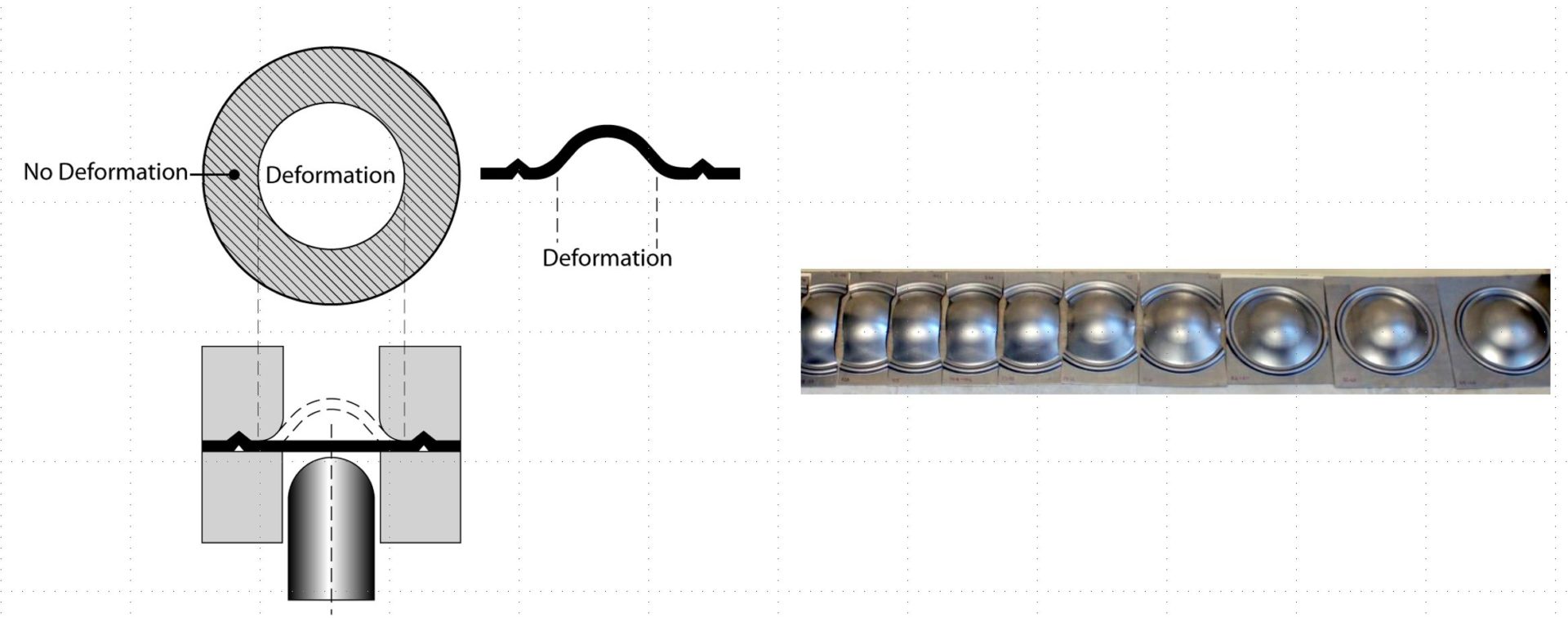
Figure 2: Forming limit curves can be created by deforming multiple samples of different widths. Narrow strips on the left allow metal to flow in from the unconstrained edges, creating a draw deformation mode leading to strains that plot on the left side of the FLC. Fully constrained samples, shown on the rightE-2, create a stretch deformation mode leading to strains that plot on the right side of the FLC.
Generally, strains are measured using one of two methods. The first approach involves covering the initially flat test samples with a grid pattern of circles, squares, or dots of known diameter and spacing to measure the strains associated with deformation. An alternate approach is based on Digital Image Correlation (DIC), where a camera tracks the movement of a random speckle pattern applied prior to forming.W-26, H-22, M-21 DIC methods are directly suited for use with stress-based FLCs.
Often, the terms Forming Limit Curve (FLC) and Forming Limit Diagram (FLD) are used interchangeably. Perhaps a better way of categorizing is to define the components and what they encompass. This is somewhat of a simplification, since detailed interactions are known to occur.
Local necking during uniaxial tensile testing limits the characterization of the stress-strain response to true strain values below uniform elongation. Extrapolating the true stress – true strain curve beyond uniform elongation requires selecting a hardening law on which to base the extrapolation. However, the chosen hardening law dramatically affects the extrapolated the true stress – true strain curve. Figure 1L-20 shows an example of this extrapolation using a bake hardenable steel. Deviation from the real performance leads to inaccurate thinning and fracture predictions, inaccurate springback predictions, and inaccurate predictions of press force and press energy requirements.

Figure 1: The selected hardening law leads to vastly different stress-strain responses extrapolated beyond uniform elongation.L-20
Bulge testing is one method to generate stress-strain data at higher strains, minimizing the need for extensive extrapolation. Another benefit is that the deformation occurs in two directions (biaxial), which is similar to the metal motion seen in most forming operations and in contrast to uniaxial tensile testing.
In biaxial bulge testingK-17, V-7, a circular sample is clamped around its periphery and pressurized from one side using a viscous incompressible medium, forcing the metal to bulge and expand into a cavity as the pressure increases. Figure 2 shows a typical testing configuration.F-12 Flow stress is calculated from the dome height of the bulging blank and the pressure in the viscous medium. A non-contact system equipped with Digital Image Correlation (DIC) measures strain. The ISO 16808 Test Standard details the requirements.I-12

Figure 2: Bulge testing configuration.F-12
For various reasons, flow stress data at the lowest strains are not as accurate as what is generated at higher strains. This leads to practitioners combining curves, using tensile data at low strains through uniform elongation, and bulge data after that. These blended curves result in a thorough true stress – true strain characterization over a wide range of strains, making it applicable to a variety of formed parts. Figure 3 shows a blended curve for the same alloy highlighted in Figure 1.

Figure 3: Flow curves for a bake hardenable steel generated by combining tensile testing with bulge testing.L-20
Biaxial bulge testing provides two critical inputs for advanced material characterizations required for simulation: biaxial anisotropy and biaxial yield stress.