![Martensite]()
1stGen AHSS, AHSS, Steel Grades
Martensitic steels are characterized by a microstructure that is mostly all martensite, but possibly also containing small amounts of ferrite and/or bainite (Figure 1 and 2). Steels with a fully martensitic microstructure are associated with the highest tensile strength – grades with a minimum specified tensile strength of 1700 MPa are commercially available, and higher strength levels are under development.

Figure 1: Schematic of a martensitic steel microstructure. Ferrite and bainite may also be found in small amounts.

Figure 2: Microstructure of MS 950/1200
To create MS steels, the austenite that exists during hot-rolling or annealing is transformed almost entirely to martensite during quenching on the run-out table or in the cooling section of the continuous annealing line. Adding carbon to MS steels increases hardenability and strengthens the martensite. Manganese, silicon, chromium, molybdenum, boron, vanadium, and nickel are also used in various combinations to increase hardenability.
The advent of water quenched lines facilitated the ability to reduce the amount of alloying additions, which has an associated benefit of producing a microstructure that is less susceptible to delayed cracking.
These steels are often subjected to post-quench tempering to improve ductility, so that extremely high strength levels can be achieved along with adequate ductility for certain forming processes like Roll Forming.
Figure 3 shows MS950/1200 compared to HSLA. Engineering and true stress-strain curves for MS steel grades are presented in Figures 4 and 5.
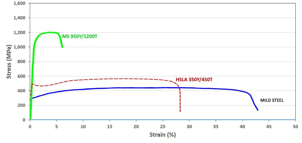
Figure 3: A comparison of stress strain curves for mild steel, HSLA 350/450, and MS 950/1200.

Figure 4: Engineering stress-strain curves for a series of MS steel grades.S-5 Sheet thicknesses: 1.8 mm to 2.0 mm.

Figure 5: True stress-strain curves for a series of MS steel grades.S-5 Sheet thicknesses: 1.8 mm to 2.0mm.
In addition to being produced directly at the steel mill, a martensitic microstructure also can be developed during the hot stamping of press hardening steels.
Examples of current production grades of martensitic steels and typical automotive applications include:
| MS 950/1200 |
Cross-members, side intrusion beams, bumper beams, bumper reinforcements |
| MS 1150/1400 |
Rocker outer, side intrusion beams, bumper beams, bumper reinforcements |
| MS 1250/1500 |
Side intrusion beams, bumper beams, bumper reinforcements |
Some of the specifications describing uncoated cold rolled 1st Generation martensite steel (MS) are included below, with the grades typically listed in order of increasing minimum tensile strength. Different specifications may exist which describe hot or cold rolled, uncoated or coated, or steels of different strengths. Many automakers have proprietary specifications which encompass their requirements.
- ASTM A980M, with Grades 130 [900], 160 [1100], 190 [1300], and 220 [1500]A-23
- VDA 239-100, with the terms CR860Y1100T-MS, CR1030Y1300T-MS, CR1220Y1500T-MS, and CR1350Y1700T-MSV-3
- SAE J2745, with terms Martensite (MS) 900T/700Y, 1100T/860Y, 1300T/1030Y, and 1500T/1200YS-18
Case Study: Using Martensitic Steels
as an Alternative to Press Hardening Steel
– Laboratory Evaluations
Martensitic steel grades provide a cold formed alternative to hot formed press hardening steels. Not all product shapes can be cold formed. For those shapes where forming at ambient temperatures is possible, design and process strategies must address the springback which comes with the high strength levels, as well as eliminate the risk of delayed fracture. The potential benefits associated with cold forming include lower energy costs, reduced carbon footprint, and improved cycle times compared with hot forming processes.
Highlighting product forms achievable in cold stamping, an automotive steel Product Applications Laboratory formed a Roof Center Reinforcement from 1.4 mm CR1200Y1470T-MS using conventional cold stamping rather than roll forming, Figure 6. Using cold stamping allows for the flexibility of considering different strategies when die processing which may result in reduced springback or incorporating part features not achievable with roll forming.

Figure 6: Roof Center Reinforcement cold stamped from CR1200Y1470T-MS martensitic steel.U-1
Cold stamping of martensitic steels is not limited to simpler shapes with gentle curvature. Shown in Figure 7 is a Center Pillar Outer, cold stamped using a tailor welded blank containing CR1200Y1470T-MS and CR320Y590T-DP as the upper and lower portion steels.U-1

Figure 7: Center Pillar Outer stamped at ambient temperature from a tailor welded blank containing 1470 MPa tensile strength martensitic steel.U-1
Another characteristic of martensitic steels is their high yield strength, which is associated with improved crash performance. In a laboratory environment, crash behavior is assessed with 3-point bending moments. A studyS-8 determined there was a correlation between sheet steel yield strength and the 3-point bending deformation of hat shaped parts. Based on a comparison of yield strength, Figure 8 shows that CR1200Y1470T-MS has similar performance to hot stamped PHS-CR1800T-MB and PHS-CR1900T-MB at the same thickness and exceeds the frequently used PHS-CR1500T-MB. For this reason, there may be the potential to reduce costs and even weight with a cold stamping approach, providing appropriate press, process, and die designs are used.

Figure 8: Effect of Yield Strength on Bending Moment. The right image shows the typical yield strength range of CR1030Y1300T-MS and CR1200Y1470T-MS as well as typical yield strength values of several Press Hardened Steels.S-8
Case Study: Martensitic Steels as an Alternative to
Press Hardening Steel – Automotive Production Examples
with Springback Mitigation Strategies
Recent years have seen some applications typically associated with press hardening steels transition to a cold stamped martensitic steel, CR1200Y1470T-MS. One such example is found in the third-generation Nissan B-segment hatchback (2020 start of production), which uses 1.2 mm thick CR1200Y1470T-MS as the material for the Second Cross Member Reinforcement.K-45
Using the carbon equivalent formula Ceq=C+Si/30+Mn/20+2P+4S K-45, the newly developed martensitic grade has a carbon equivalent value of 0.28, which is lower than the 0.35 associated with the conventional PHS grade of comparable tensile strength, 22MnB5 (PHS 1500T). The lower carbon equivalent value is expected to translate into easier welding conditions. Furthermore, conventional mechanical trimming and piercing equipment and techniques work with the cold formable martensitic grade, whereas parts formed from press hardening steels typically require laser trimming or other more costly approaches. An evaluation of delayed fracture found no evidence of this failure mode.
Figure 9 highlights this reinforcement, with its placement on the cross member and in the vehicle shown in red. The varying elevation of this part, combined with a non-uniform cross section at the outermost edges, help control springback, but makes roll forming significantly more challenging if that were the cold forming approach.

Figure 9: Cold-Stamped Martensitic Steel with 1500 MPa Tensile Strength used in the Nissan B-Segment Hatchback.K-57
Unbalanced stresses in stamped parts lead to several types of shape fixability issues collectively called springback. In hat shape wall sections, shape fixing beads sometimes referred to as stake beads (see Post Stretch information at this link) mitigate sidewall curl by imparting a tensile stress state on both the top and bottom sheet surfaces and increasing the rigidity. Springback control to limit flexing down the length of longitudinally curved parts requires a different technique. Here, the root cause is the stress difference between the tensile stress at the punch top and the compressive stress at the flange at bottom dead center of the press stroke. Figure 10 presents schematics of the stress distribution when the punch is located at bottom dead center of the press stroke, and the shape fixability issue after load removal.

Figure 10: Cold-Stamped Martensitic Steel With 1500 MPa Tensile Strength Used in the Lexus NXJ-24
A patented approach known as Stress Reverse Forming™T-44 improved dimensional accuracy in the second-generation Lexus NX (2021 start of production) center roof reinforcement, cold stamped from martensitic steel, CR1200Y1470T-MS.J-24 Figure 11 shows different views of this part.

Figure 11: Left Image: Springback Differences Exist in Coils at the Low and High End of the Strength Specification; Right Image: Stress Reverse Forming™ Process Reduces Sensitivity to Springback (Images Adapted from Citation T-29)
Stress Reverse Forming™T-44 uses the principles of the Bauschinger Effect to reverse the direction of the forming stresses during a restrike forming process to achieve a final part closer to the targeted dimensions.T-29 Parts processed with this two-step approach are first over-formed to a smaller radius of curvature than the final part shape. Removing the part from the tool after this first forming step results in the stress distribution seen in the left image in Figure 10. The unique aspect of this approach comes from the second forming step where the tool shape forces the punch top into slight compression while the lower flange is put into slight tension. The tool shape used in this stage contains a slightly greater radius of curvature than the targeted part shape. As shown in Citation T-29, this process appears to be equally effective at all steel strengths.
Without effective countermeasures, springback increases with part strength. Related to this is the springback difference between coils having strength at the lowest and highest ends of the acceptable property range. This can lead to substantial differences in springback between coils completely within specification. However, after using effective countermeasures such as Stress Reverse Forming™ described in Citation T-29, springback differences between coils are minimized, which leads to increased dimensional accuracy and more consistent stamping performance. This phenomenon is shown schematically in Figure 12. Furthermore, unlike conventional stamping approaches, the amount of springback in parts made with this approach does not increase with steel strength.

Figure 12: Left Image: Springback Differences Exist in Coils at the Low and High End of the Strength Specification; Right Image: Stress Reverse Forming™ Process Reduces Sensitivity to Springback (Images Adapted from Citation T-29)

Blog, homepage-featured-top, main-blog
One of the tasks we took great care in completing during the update of the AHSS Application Guidelines was to provide a definition for what constitutes a third generation (3rd Gen) Advanced High-Strength Steel. We had been asked this question many times, and often in addressing the question among our technical editors, we would get various responses. Consequently, we made it a part of a discussion with our AHSS Guidelines Working Group, made up of steel subject matter experts from around the world at our member companies. The following article reflects the outcome of that discussion and is the definition adopted by WorldAutoSteel.
First Generation Advanced High-Strength Steels (AHSS) are based on a ferrite matrix for baseline ductility, with varying amounts of other microstructural components like martensite, bainite, and retained austenite providing strength and additional ductility. These grades have enhanced global formability compared with conventional high strength steels at the same strength level. However, local formability challenges may arise in some applications due to wide hardness differences between the microstructural components.
The Second Generation AHSS grades have essentially a fully austenitic microstructure and rely on a twinning deformation mechanism for strength and ductility. Austenitic stainless steels have similar characteristics, so they are sometimes grouped in this category as well. 2nd Gen AHSS grades are typically higher-cost grades due to the complex mill processing to produce them as well as being highly alloyed, the latter of which leads to welding challenges.
Third Generation (or 3rd Gen) AHSS are multi-phase steels engineered to develop enhanced formability as measured in tensile, sheared edge, and/or bending tests. Typically, these steels rely on retained austenite in a bainite or martensite matrix and potentially some amount of ferrite and/or precipitates, all in specific proportions and distributions, to develop these enhanced properties.
Individual automakers may have proprietary definitions of 3rd Gen AHSS grades containing minimum levels of strength and ductility, or specific balances of microstructural components. However, such globally accepted standards do not exist. Prior to 2010, one steelmaker had limited production runs of a product reaching 18% elongation at 1000 MPa tensile strength. Starting around 2010, several international consortia formed with the hopes of achieving the next-level properties associated with 3rd Gen steels in a production environment. One effortU-11, S-95 targeted the development of two products: a high strength grade having 25% elongation and 1500 MPa tensile strength and a high ductility grade targeting 30% elongation at 1200 MPa tensile strength. The “exceptional-strength/high-ductility” steel achieved 1538 MPa tensile strength and 19% elongation with a 3% manganese steel processed with a QP cycle. The 1200 MPa target of the “exceptional-ductility/high-strength” was met with a 10% Mn alloy, and exceeded the ductility target by achieving 37% elongation. Another effort based in EuropeR-22 produced many alloys with the QP process, including one which reached 1943 MPa tensile strength with 8% elongation. Higher ductility was possible, at the expense of lower strength.
3rd Gen steels have improved ductility in cold forming operations compared with other steels at the same strength level. As such, they may offer a cold forming alternative to press hardening steels in some applications. Also, while 3rd Gen steels are intended for cold forming, some are appropriate for the hot stamping process.
Like all steel products, 3rd Gen properties are a function of the chemistry and mill processing conditions. There is no one unique way to reach the properties associated with 3rd Gen steels – steelmakers use their available production equipment with different characteristics, constraints, and control capabilities. Even when attempting to meet the same OEM specification, steelmakers will take different routes to achieve those requirements. This may lead to each approved supplier having properties which fall into different portions of the allowable range. Manufacturers should use caution when switching between suppliers, since dies and processes tuned for one set of properties may not behave the same when switching to another set, even when both meet the OEM specification.
There are three general types of 3rd Gen steels currently available or under evaluation. All rely on the TRIP effect. Applying the QP process to the other grades below may create additional high-performance grades.
- TRIP-Assisted Bainitic Ferrite (TBF) and Carbide-Free Bainite (CFB)
- TRIP-Assisted Bainitic Ferrite (TBF) and Carbide-Free Bainite (CFB) are descriptions of essentially the same grade. Some organizations group Dual Phase – High Ductility (DP-HD, or DH) in with these. Their production approach leads to an ultra-fine bainitic ferrite grain size, resulting in higher strength. The austenite in the microstructure allows for a transformation induced plasticity effect leading to enhanced ductility.
- Quenched and Partitioned Grades, Q&P or simply QP
- Quenching and Partitioning (Q&P) describes the processing route resulting in a structure containing martensite as well as significant amounts of retained austenite. The quenching temperature helps define the relative percentages of martensite and austenite while the partitioning temperature promotes an increased percentage of austenite stabile room temperature after cooling.
- Medium Manganese Steels, Medium-Mn, or Med-Mn
- Medium Manganese steels have a Mn content of approximately 3% to 12%, along with silicon, aluminum, and microalloying additions. This alloying approach allows for austenite to be stable at room temperature, leading to the TRIP Effect for enhanced ductility during stamping. These grades are not yet widely commercialized.
We have much more information on 3rd Gen steels here in the Guidelines. Take a look at the full 3rd Generation Steels article for much more detail on the three types listed above.
Blog, homepage-featured-top, main-blog
The rule of thumb estimates used in 1989 during my internship with an automotive stamping supplier were simple calculations for the peak load. Tonnage for trim and pierce operations depended on the length of line of trim, material thickness and the shear strength of the material. Tonnage for forming operations depended on the size of the form, material thickness and material tensile strength. These calculations typically over-predicted the tonnage requirement, but due to the relatively low strength compared to AHSS, the overall part size that dictated the required press size became the limiting factor rather than the tonnage requirement.
Applying these same rules of thumb to the advanced steels in use today will likely under-predict the tonnage requirements. To understand why, let us examine the guidelines I used over 30 years ago.
For piercing a hole: Tonnage = d * t * 80 Equation 1
In this equation d is the punch diameter in inches, t is the material thickness in inches, and it calculates tonnage in tons. This was a simple and effective way to estimate the tonnage of all the holes pierced. Equation 1 is a simplification of the proper calculation being the length of line doing the work, in this case the circumference of a circle, multiplied by the sheet thickness and the material’s shear strength (ꚍ). The generic equation for any type of piercing or trimming is Tonnage = P * t * ꚍ where P is the perimeter or length of line of the trim, t is the sheet thickness and ꚍ is the shear strength of the material. A typical estimate for the shear strength (ꚍ) of mild steel is 60% of the tensile strength (T). Therefore, the equation development for a simple hole piercing looks like:
| Generic trim equation: |
Tonnage = P * t * ꚍ |
Equation 2 |
| Specific for a round hole: |
Tonnage = πd * t * 0.6T |
|
| Simplifying: |
Tonnage = d * t * 0.6Tπ |
|
| Mild steel T = 300 MPa = 43.5 ksi: |
0.6 * 43.5 * 3.14 = 82 |
|
| Pierce a round hole: |
Tonnage = d * t * 80 |
|
Knowing how the rule of thumb was derived allows us to highlight some possible sources of error. First, the equation assumes trimming of the full thickness. In reality, a typical trim operation for steel consists of 20% to 50% trimming and the remainder is breakage. The press needs to apply load only for the trimming portion. Second, shear strength is not a fixed percentage of tensile strength. The actual shear strength should be measured for each specific grade as the microstructure differences of the AHSS will affect the material strength in shear. Lastly each of these errors are multiplied since today’s AHSS material has a tensile strength of three to five times that of mild steel. To see this, we can consider a simple example of piercing a 1-inch hole in 0.06 inch (1.5 mm) thick mild steel. Mild steel tensile strength typically ranges from 40 ksi to 55 ksi (280 MPa to 380 MPa). Looking at Equation 1 relative to Equation 2 with low- and high -end assumptions:
| Equation 1 estimate |
Tonnage = 1 * 0.06 * 80 = 4.8 tons |
| Equation 2 minimum |
Tonnage = 3.14 * 0.06(20%) * 0.6(40) = 0.9 tons |
| Equation 2 maximum |
Tonnage = 3.14 * 0.06(50%) * 0.6(55) = 3.1 tons |
This simple example shows sources of error that could lead to an estimate ranging from 0.9 to 4.8 tons to pierce a single hole. A similar exercise could apply to a drawing operation. In this situation, most rules of thumb attempt to use the perimeter or surface area of the part, the material thickness and the material tensile strength to predict the tonnage needed. Sources for error in this type of calculation include: 1) Using the perimeter of the draw area, tending to under-predict; 2) Using the surface area of the part, tending to over-predict; and 3) Using the tensile strength of the material, also tending to over-predict as it assumes the material is stretched right to the level of splitting. Correction factors have been developed over time, but it is still easy to see there are many possible sources of error in these types of calculations.
AHSS Magnifies Press Tonnage Prediction Challenges
A number of reasons explain why the inherent challenges with old-school rules of thumb are exaggerated with AHSS:
- Strength: The strength of today’s cold stamped steels is quite incredible. Where a mild steel may have a tensile strength of 280 MPa, it is now common to cold stamp dual phase (DP) steels and 3rd Generation steels with up to 1180 MPa. In addition, new materials having a tensile strength of 1500 MPa with enough elongation to allow for cold stamping are starting to enter the market. This five-fold increase in strength acts as a multiplying factor for any errors in traditional predictions.
- Formability: The formability of AHSS has also increased dramatically. Today a DP 590 steel and even a 980 3rd Generation steel can have nearly the same elongation as a high-strength low alloy (HSLA) steel of 30 years ago. This affords the part designers the ability to incorporate more complex forms into a part including using darts and beads to increase a part’s stiffness, tight radii and deeper draws. All of these add to the tonnage used and are generally not part of the old school rule of thumb calculations.
- Springback Corrections: Springback is linearly related to the yield strength of a material. Therefore, stamping AHSS grades require more features to be added to the die process to control springback. These may include draw beads (used to control material flow early in the press stroke), stake beads (used at the bottom of the stroke to minimize springback) and tighter radii (Figure 2). These features are typically off product, in the addendum, and are easily ignored by typical rule of thumb calculations.

Figure 2: Draw and Stake Bead PlacementA-6
- Hardening Curves: The complex microstructure of AHSS offers many advantages to increase formability. All AHSS grades produce microstructural phase transformations during the stamping process. This allows the lower yield strength in the as-rolled material, which aids in formability, to increase during the stamping operation. This yield strength increase can be as much as 100 MPa. Models that estimate these hardening curves of the material are ignored when doing hand calculations.
- Other Considerations: Lastly the typical rule of thumb calculations, as we have discussed, only consider the part characteristics. They generally do not include the other sources that consume energy during the stamping process including off-product feature (beads, pilot holes, etc.), spring stripper pressure, pad pressure from nitrogen springs or air cushions, driven cams and part lifters. Many of these could be ignored 30 years ago with mild steels, but they become more significant with the strength of today’s AHSS.
Next Steps
Accurately predicting press requirements is a decades-long, industry-wide issue. Auto/Steel Partnership (A/SP), a partnership between automotive OEMs, steel mills and affiliate suppliers, teamed up with formability software suppliers to improve press tonnage prediction accuracy. A/SP’s efforts, including this project, looks to bridge the gap between research laboratories and the shop floor.
Stamping companies should keep press tonnage monitors in good working order, and upgrade to systems that can capture full through-stroke force curves. Engaging with organizations like A/SP, OEMs and steel mills, allows efficient information sharing and capturing best-practices. Get the steel mill involved early, even in the die design phase. All steel mills have teams of application engineers to help OEMs and their suppliers transition into using the newest grades of steel – they want stampers to succeed and have the tools and data to help.
Read more about Press Tonnage Prediction in the expanded article.
Blog, homepage-featured-top, main-blog
Advanced High-Strength Steel (AHSS) products have significantly different forming characteristics and these challenge conventional mechanical and hydraulic presses. Some examples include the dramatically higher strength of these new steels resulting in higher forming loads and increased springback. Also, higher contact pressures cause higher temperatures at the die-steel interface, requiring high performance lubricants and tool steel inserts with advanced coatings.
These and other challenges lead to issues with the precision of part formation and stamping line productivity. Using a servo-driven press is one approach to address the challenges of forming and cutting AHSS grades. Recent growth in the use of servo presses in the automotive manufacturing industry parallels the increased use of AHSS in the body structure of new automobiles. Click to read more about the Characteristics of Servo Presses and their Advantages.
Figure 1 shows the difference between the available motions of flywheel-driven mechanical presses verses servo driven mechanical presses. The slide motion of the servo press can be programmed for more parts per minute, decreased drawing speed to reduce quality errors, or dwelling or re-striking at bottom dead center to reduce springback.

Figure 1: Comparison of Press Signatures in Fixed Motion Mechanical Presses and Free-Motion Servo-Driven Presses.M-3
Press Force and Press Energy
Categorizing both mechanical and hydraulic presses requires three different capacities or ratings – force, energy, and power. Historically, when making parts out of mild steel or even some HSLA steels, using the old rules-of-thumb to estimate forming loads was sufficient. Once the tonnage requirements and some processing requirements were known, stamping could occur in whichever press met those minimum tonnage and bed size requirements.
In these cases, press capacity (for example, 1000 kN) is a suitable number for the mechanical characteristics of a stamping press. Capacity, or tonnage rating, indicates the maximum force that the press can apply without damaging its components, like the machine frame, slide-adjusting mechanisms, pitman (connection rods) or main gear bushings.
A servo press transmits force (not energy) the same way as the equivalent conventional press (mechanical or hydraulic). However, the amount of force available throughout the stroke depends on whether the press is hydraulic or mechanically driven. Hydraulic presses can exert maximum force during the entire stroke as tonnage generation occurs via hydraulic fluid, pumps, and cylinders. Mechanical presses exert their maximum force at a specific distance above bottom dead center (BDC), usually defined at 0.5 inch. At increased distances above bottom dead center, the loss of mechanical advantage reduces the tonnage available for the press to apply. This phenomenon is known as de-rated tonnage, and it applies to conventional mechanical presses as well as servo-mechanical presses. Figure 2 shows a typical press-force curve for a 600-ton mechanical press. In this example, when the press is approximately 3 inches off BDC, the maximum tonnage available is only 250 tons – significantly less than the 600-ton rating.

Figure 2: The Press-Force curve shows the maximum tonnage a mechanical press can apply based on the position of the slide relative to the bottom dead center reference distance. This de-rated tonnage applies to both conventional mechanical presses as well as servo-mechanical presses.E-2
Press energy reflects the ability to provide that force over a specified distance (draw depth) at a given cycle rate. Figure 3 shows a typical press-energy curve for the same 600-ton mechanical press. The energy available depends on the size and speed of the flywheel, as well as the size of the main drive motor. As the flywheel rotates faster, the amount of stored energy increases, reflected in the first portion of the curve. The cutting or forming process consumes energy, which the drive motor must replenish during the nonworking part of the stroke. At faster speeds, the motor has less time to restore the energy. If the energy cannot be restored in time, the press stalls. The graph illustrates how the available energy of the press diminishes to 25% of the rated capacity when accompanied by a speed reduction from 24 strokes per minute to 12 strokes per minute.

Figure 3: A representative press-energy curve for a 600 ton mechanical press. Reducing the stroke rate from 24 to 12 reduces available energy by 75%.E-2
Case Study: Press Force and Press EnergyH-3
Predicting the press forces needed initially to form a part is known from a basic understanding of sheet metal forming. Different methods are available to calculate drawing force, ram force, slide force, or blankholder force. The press load signature is an output from most forming-process development simulation programs, as well as special press load monitors. The topic of press force predictions will be covered in this Blog in the months ahead.
Most structural components include design features to improve local stiffness. Typically, forming of the features requiring embossing processes occurs near the end of the stroke near Bottom Dead Center. Predicting forces needed for such a process is usually based on press shop experiences applicable to conventional steel grades. To generate comparable numbers for AHSS grades, forming process simulation is recommended.
In Citation H-3, stamping simulations evaluated the forming of a cross member having a hat-profile with an embossment formed at the end of the stroke (Figure 4). The study simulated press forces and press energy involved for drawing and embossing a channel section from four steel grades approximately 1.5 mm thick: mild steel, HSLA 250/350, HSLA 350/450, and DP 350/600. Figures 5A and 5B clearly show that the embossing phase rather than the drawing phase dominates the total force and energy requirements, even though the punch travel for embossing is only a fraction of the drawing depth.

Figure 4: Cross section of a component having a longitudinal embossment to improve local stiffness.H-3
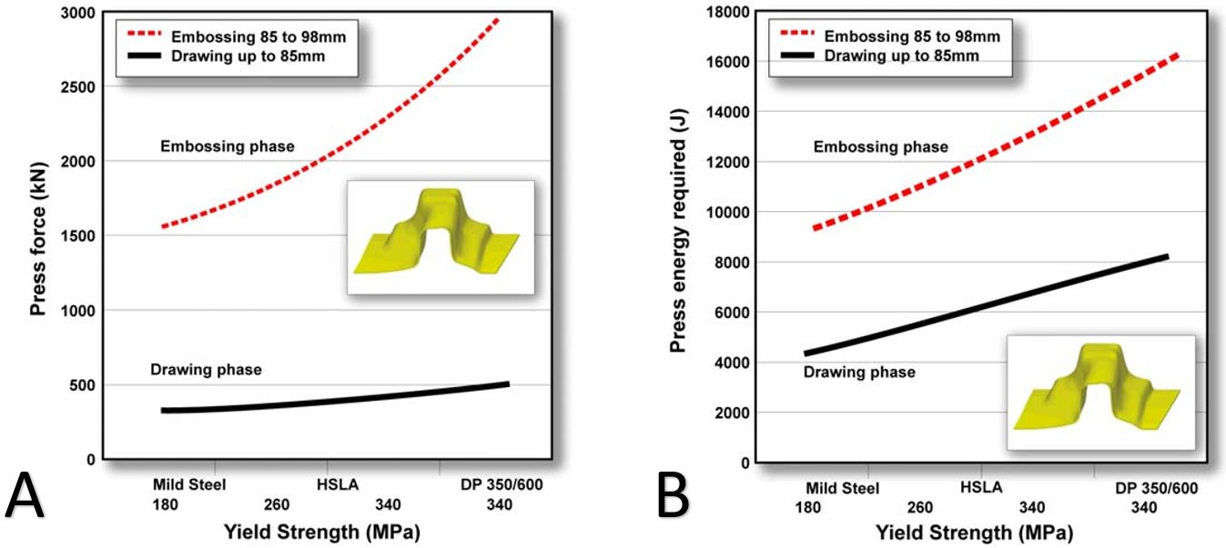
Figure 5: Embossing requires significantly more (A) force and (B) energy than drawing, even though the punch travel in the embossing stage is much smaller.H-3
Figures 6 and 7 highlight the press energy requirements, showing the greater energy required for higher strength steels. The embossment starts to form at a punch displacement of 85 mm, indicated by the three dots in Figure 6. The last increment of punch travel to 98 mm requires significantly higher energy, as shown in Figure 7. Note that compared with mild steel, the dual phase steel grade requires significantly more energy to form the part to home with the 98 mm travel.

Figure 6: Energy needed to form the component increases for higher strength steel grades. Forming the embossment begins at 85 mm of punch travel, indicated by the 3 dots.H-3

Figure 7: Additional energy required to form the embossment increases for higher strength steel grades.H-3
It is not only embossments that require substantially more force and energy at the end of the stroke. Stake beads for springback control engage late in the stroke to provide sidewall stretch. Depending on the design of the forming process, the steel into which the stake beads engage may have passed through conventional draw beads for metal flow control, and therefore are work-hardened to an even higher strength. This leads to greater requirements for die closing force and energy. Certain draw-bead geometries which demand different closing conditions around the periphery of the stamping also may influence closing force and energy requirements.
A more detailed Press Requirements article contains additional information and case studies. Read it here >>>

Resistance Welding Steel to Aluminium
This article summarizes a paper entitled, “Process, Microstructure and Fracture Mode of Thick Stack-Ups of Aluminum Alloy to AHSS Dissimilar Metal Spot Joints”, by Luke Walker, Colleen Hilla, Menachem Kimchi, and Wei Zhang, Department of Materials Science and Engineering, The Ohio State University.W-9
Researchers at The Ohio State University studied the effects of adding a stainless steel (SS) insert to a dissimilar Advanced High-Strength Steel (AHSS) to aluminum (Al) resistance spot weld (RSW). The SS insert was ultrasonically welded to the Al sheet prior to the RSW being performed. The purpose of the SS is to reduce the intermetallic layer that forms when welding steel to aluminum. This process increases the strength and toughness of the weld. In this study, the process is applied to three sheet (3T) stack up that contains one Al sheet and two 1.2 mm thick Press Hardened (PH) 1500 sheets. The joint strength is measured in lap shear testing and the intermetallic thickness/ morphology is studied after cross sectioning the welds.
During the microstructure evaluation it was noted that Al 6022 contained a larger nugget diameter as compared to the Al 5052 welds. A few potential reasons for the hotter welds were proposed including cleanliness of the electrodes, surface oxides, and thickness of the different alloys. The welds on the Al 5052 stack ups were made first on clean electrodes whereas the Al 6022 was made on potentially dirty electrodes that increased the contact resistance. The effects of different surface oxides are not likely given the SS sheet is ultrasonically welded but could still add to the higher heat input in the RSW. The Al 6022 is 0.2 mm thicker, which could increase the bulk resistance and decrease the cooling effect from the electrodes.
The 3T welds likely had much lower strength and toughness due to cracks that formed at the Al-SS insert interface. These can be attributed to an increase in intermetallic compound (IMC) thickness and the residual stress caused by the forge force. The IMC thickness was measured two ways: The first measurement was of the continuous IMC layer and the second was from the Al-Fe interface to the end of the IMC dendrites (Figure 1, 2 and Table 1). The Al 5052 observed the thickest continuous IMC layer but Al 6022 was close to the Al 5052 thickness. This can be attributed to the increased Si content of Al 6022 which has been shown to decrease the growth of Fe-Al intermetallics.
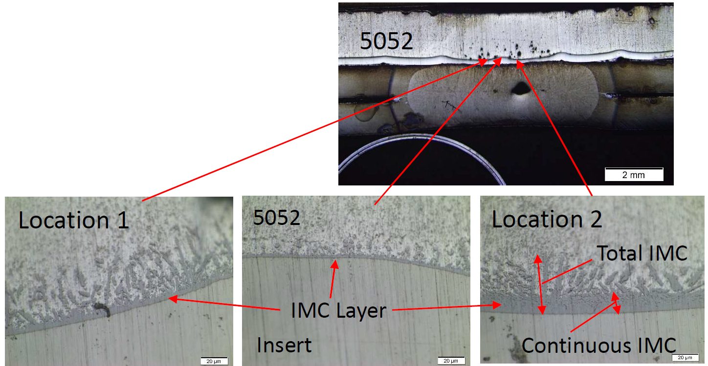
Figure 1: IMC in the Al Alloy 5052 to Stainless-Steel Weld.W-9
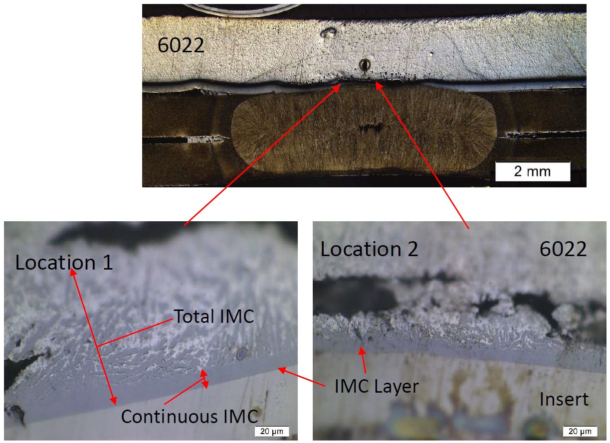
Figure 2: IMC in the Al Alloy 6022 to Stainless-Steel Weld.W-9
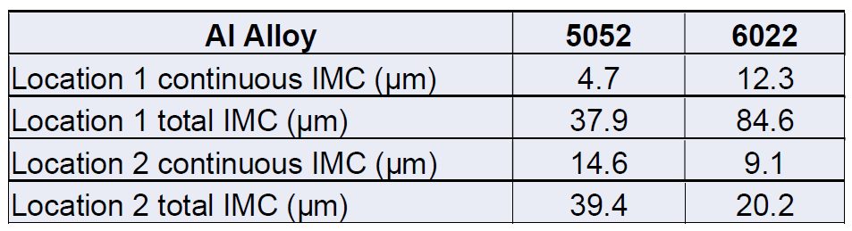
Table 1: IMC Thickness of Both the 5052 Weld and the 6022 Weld.W-9
Referencing Figure 3, the 2T stack-up has a higher tensile strength as well as significantly higher fracture energy absorbed compared to the 3T stack-ups. This is mainly attributed to the failure mode observed in the different stack-ups. The 2T welds had button pullout failure while 3T stack-ups had interfacial Failure.
![Figure 3: Failure Load and Fracture Energy [(A) Al to steel (Al-Us) welds and (B) steel to steel (Us-Us) welds (the 2T 6022 results are from previous work(10))]W-9](https://ahssinsights.org/wp-content/uploads/2021/12/fig4-process.jpg)
Figure 3: Failure Load and Fracture Energy [(A) Al to steel (Al-Us) welds and (B) steel to steel (Us-Us) welds (the 2T 6022 results are from previous work(10))]W-9
The Al 6022 contains higher Si content which likely decreased the growth of the continuous IMC layer but not the overall IMC layer (as seen in Figure 4 and Figure 5) due to higher weld temperatures. The joint strength of the welds in the 3T stack-ups were closer to the expected weld strength unless there was expulsion that caused a 5-kN drop in strength.
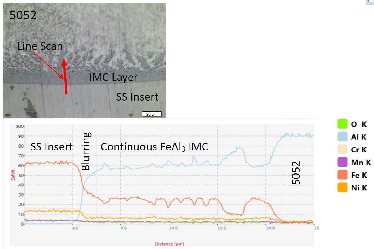
Figure 4: EDS Line Scan of the IMC in Location 2 on the 5052 3T Sample (SS stands for austenitic stainless steel 316).W-9
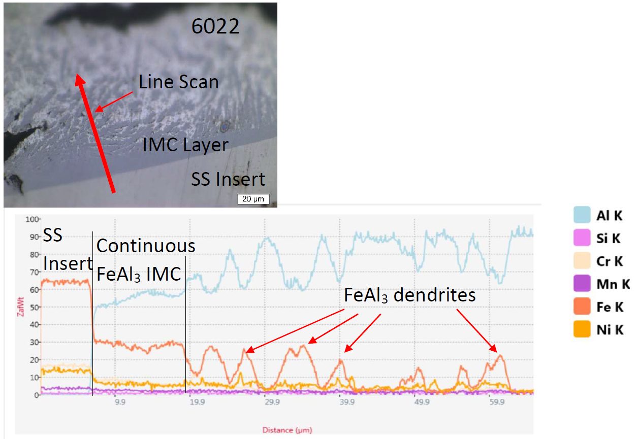
Figure 5: EDS Line Scan of the Intermetallic Layer at Location 1 on the 6022 3T Sample (SS stands for austenitic stainless steel 316).W-9