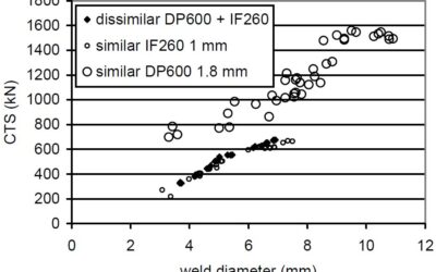
This article summarizes a paper entitled, "Higher than Expected Strengths from Dissimilar Configuration Advanced High-Strength Steel Spot Welds", by E. Biro, et al.B-6 This study shows that the cross tension strength (CTS) is always higher than the strength expected...
Higher than Expected Strengths
read more