Joining, Projection Welding
As with resistance spot welding in automotive applications, projection welding also is used to join two overlapping sheets of relatively thin metal. The process involves pressing a projection or number of projections in one of the plates and welding the two plates together at the projection locations.
The method can also be used for welding metal sheet to the ends of bars, rods or pipes, or for welding bolts, nuts, and other attachments to sheets. Such attachments are being used widely in the automotive industry. Wire grids (i.e. the crossing points of the wires) are also particularly suitable for projection welding (it is also called cross wire welding).
A modern car body may contains some 300 welded and punched fasteners, such as bolts, nuts, and studs. The quality of the attachment of these fasteners to the stamped body components is critical for the final product’s safety and reliability. Crucial components such as the front and rear axles are mounted to such fasteners, the seat belts and steering column are anchored to them, and they provide grounding for electrical wires.L-25
As noted, projection welding is similar to resistance spot welding. However, in the Resistance Spot Welding process, the size of the contact surface of the electrode cap tip determines the current flow, whereas in projection welding, the current flow is constricted to the embossed or machined projection as shown in Figure 1. Both AC and DC power sources are suitable for fastener welding. The heat balance for projection welding is affected by the following factorsA-11:
- Projection design and location
- Thickness of the sheet to which the fastener is attached
- Thermal and electrical conductivities of the metals being welded
- Heating rate
- Electrode alloy type
As compared to Resistance Spot and Seam Welding, Resistance Projection Welding is capable of welding much thicker parts, as well as parts with a significant thickness mismatch. As a result, it is often considered as a potential replacement for arc welding processes such as GMAW. One of the reasons for this is the drastic reduction in welding time that can be achieved. For example, a typical automotive part that might require several minutes or more of welding with the GMAW process may have the potential to be welded in less than a few seconds with the Resistance Projection Welding process. This is because the entire weld or multiple welds can be made at the same time in a single fixture. Another advantage of the process, relative to spot welding, is that there is less wear and tear on the electrodes.
Different types of projections made by different methods are shown in Figure 2. It is important to note that the types of projections that are extensions of the part are known as solid projections (2-B and 2-D) and can only be produced by a machining or forging process, whereas the other projections are more easily produced by stamping with a punch and die. Projections produced with a punch and die usually involve the formation of a molten nugget during welding but not always. The solid projection designs mostly result in solid‐state welds that occur via a forging action as the projection is heated and pressure applied. A common Projection Welding application that uses solid projections involves the attachment of a wide variety of nuts, bolts, and fasteners. Many fasteners used on automobiles are attached this way.

Figure 1: Welding current flow concentration due to projection geometry.

Figure 2: Typical projection types and designs.
RSW Parameter Guidelines
This article summarizes a paper entitled, “RSW of 22MnB5 at Overlaps with Gaps-Effects, Causes, and Countermeasures”, by J. Kaars, et al.K-12
This study aims to elaborate on the influencing mechanisms of gaps on the welding result. Welding experiments at artificial gaps and finite element analysis (FEA) of the welding process have been used to investigate the matter. In both methods, the same configuration of two 1.5-mm-thick 22MnB5+AS150 welded with electrodes of the type ISO 5821 B0-16-20-40-6-30 was considered. Tensile tests yielded an ultimate tensile strength (UTS) of the press-hardened material of 1481 ± 53 MPa with a strain to fracture of 7.5 ± 0.26%. A microsection of the coating morphology after heat treatment can be found in Figure 1.

Figure 1: Morphology of the Aluminum-Silicon Coating.K-12
To set up an artificial and reproducible gap between the sheets, a dedicated fixture was used. It is displayed in Figure 2. All welding experiments were carried out with a 6-kN electrode force.

Figure 2: Fixture for Welding at Artificial Gaps, Definition of Quantities.K-12
In Table 1, the parameter variations of the gaps investigated in this work are presented.

Table 1: List of Gap Parameters Investigated.K-12
A 7-kN maximum denting force was observed at the gap (10|60). With a gap of (10|40) the gap could not be closed with the machines’ 8-kN clamping force capacity. In comparative tests on mild steel for deep drawing a clamping force of about 2 kN was required to overcome the gap (10|60) (see Figure 3). The main effects diagram of the denting force clearly shows that the average denting force gets smaller with increasing support width and becomes larger with increasing gap clearance.

Figure 3: Main Effects Diagram of the Denting Force.K-12
In Figure 4, the achieved nugget diameters at different gaps using a constant machine setting of Iw,f = 6.4 kA are displayed.

Figure 4: Effect of Gaps on Nugget Diameter, Absolute and Relative Results.K-12
A two-staged welding program, starting with a preheat current followed by a larger finishing current proved to yield the best welding results with the material used, cf., Figure 5. In Figure 5, the applied welding current program along with the measured and computed total resistance curve is displayed.

Figure 5: Exemplary Total Resistance Curve of a Weld without Gap, Measured and Computed Results.K-12
The FEA model can represent the welding process in terms of nugget diameter, dynamic resistance curve, and total electric energy with great accuracy. In Figure 6, the partial resistances of the weld as computed by FEA are composed.

Figure 6: Partial Electrical Resistances at Different Gap Configurations.K-12
In the top section of Figure 7, the computed sheet thickness curve during the process for different gaps is presented. Increased electrode indentation during welding at gaps is the reason for reduced resistance and, therefore, results in reduced nugget diameters. The lower section of Figure 7 shows the plastic strains in the sheets along with a visibly reduced sheet thickness.

Figure 7: Dynamic Sheet Thickness (up) and Plastic Strain in millimeters at Different Gaps (low, to scale).K-12
Additional welding experiments were performed to clarify, if increased welding current can counter the gap effect and maintain the energy level of the weld. The results are shown in Figure 8. They prove that increased weld current is sufficient to not only maintain the nugget diameter at gaps, but moreover increase it.

Figure 8: Nugget Diameter and Energy of Spot Welds near the Splash Limit at Overlaps with Gap.K-12
Results of further investigations on the weldability lobe of the joint are composed in Figure 9.. It is visible that with increasing gap the current range shifts toward larger currents and gets narrower.
RSW Joint Performance Testing
This articles summarizes a paper entitled, “New Test to Analyze Hydrogen Induced Cracking Susceptibility in Resistance Spot Welds,” by M. Duffey.D-10
This study aims to develop a new weldability test to analyze the susceptibility of HIC in RSW of different steels. A total of eight different steel samples were analyzed with their carbon content, associated American Welding Society (AWS) carbon equivalencies, and gauges shown in Table 1. All materials were tested in the full-hard condition (all have been cold-rolled).

Table 1: Tested Steels, Carbon Equivalencies, and Steel Gauge.D-10
The associated parameter ranges for welds made with each steel are in Table 2. The resistance spot weld was made in the middle of the sheets, as shown in the test setup in Figure 1. There was a total of 18 test samples (nine not painted and wiped, nine painted) for each material tested.

Table 2: Welding Parameters.D-10

Figure 1: HIC Test for Resistance Spot Welds Schematic.D-10
Figure 2A shows the results of the 3- × 3-in. tests. Figure 2B shows the results of the 4- × 4-in. tests. Figure 2C shows the results of the 5- × 5-in. tests.

Figure 2: Results of the Three Different Test Sizes on AHSS.D-10
Cracks consistently initiated at the periphery of the weld nugget where the two steel sheets came together. Cracks then propagated either in the weld metal or HAZ, as shown in Figures 3 and 4.

Figure 3: Cracking in the Weld Metal of Steel 8.D-10

Figure 4: Cracking in Both the Weld Nugget and HAZ in Steel 8.D-10
Figure 5 displays the results from Steels 1, 4, and 5. Steel 1 is the most resistant (of the three) to HIC. For the three steels shown in Figure 5, the crack length (at each gap spacing) was longer for the painted sample than the non-painted sample.

Figure 5. Test Results for Steels 1, 4, and 5.D-10
The microstructure of IF Steels 1-3 (Figure 6A) was ferrite. The microstructure of the high-strength low-alloy (HSLA) Steel 4 (Figure 6B) was a mixture of grain boundary ferrite, martensite, and possibly some bainite. The microstructure of the specialty alloy Steels 5-7 and AHSS Steel 8 (Figure 6C) was entirely martensite.

Figure 6: Microstructures of the Different Weld Nuggets.D-10
Figure 7 shows the fracture surface of a crack completely through Steel 7.

Figure 7: Fracture Surface of Cracked Weld in Steel 7.D-10
The average and maximum hardness results of spot welds in each material are summarized in Figure 8.

Figure 8. The Average and Maximum Hardness of HAZ and Weld Nugget in Resistance Spot Welds of Each Steel.D-10
Figure 9 is a graph that displays the carbon equivalence, number of washers where cracking first began, and average hardness of the weld nugget and HAZ in each steel.

Figure 9: Carbon Equivalency vs. Number of Washers to Initiate Cracking.D-10
Projection Welding
placeholder
Projection Welding
This paper summarizes a paper, entitled “Resistance Welding Projection Methodologies as Applied to Hot-Stamped Boron”, by D. Crist, et al.C-11
The study focuses on two different Resistance Projection Welding approaches and compares the welding parameters, mechanical properties and destructive results. Table 1 lists the secondary impedance measurements and Table 2 lists the material information for the PHS-CR1500T-MB-AS.

Table 1: Secondary Impedance Measurements.C-11

Table 2: Coupon Material Information.C-11
The thickness of the material chosen was 1.80 mm and the weld coupon dimensions are shown in Figure 1.

Figure 1: Weld Coupon Dimensions (not to scale).C-11
The projection weld nut used for testing is an M6 hex flange, three projections, non-piloted weld fastener. Detailed dimensions are shown in Figure 2.

Figure 2: Projection Weld Nut.C-11
Table 3 lists the weld schedule methodologies tested in this study. Table 4 shows the optimized weld schedules based upon push-off strength and visual weld flash level.

Table 3: Weld Schedule Development.C-11

Table 4: Optimized Weld Schedules.C-11
Repeatability testing for both Methods A and B are shown in Figures 3 and 4. The data produced for Method B shows a higher average of repeatability.

Figure 3: Repeatability Push-Off Method A.C-11

Figure 4: Repeatability Push-Off Method B.C-11
Two different failure methods were observed. Figure 5 shows full thickness buttons were pulled thought the flange for Method A and Figure 6 demonstrates partial thickness failure for Method B.

Figure 5: Method A (17.0 kA, 100 ms, 1000 lb.) Common Failure Mode.C-11

Figure 6: Method B (35.0 kA, 14 ms, 2500 lb.) Common Failure Mode.C-11
Figure 7 shows the microhardness traverse results for both Methods A and B. Method A yields a much larger HAZ. Method B shows a much smaller HAZ, less impact on the base material, and appears to be a solid state bond.

Figure 7: Microhardness Traverse.C-11
Projection Welding
This article summarizes a paper entitled, “Weld Quality Study of Projection Nut Welding with Modular Weld Head”, by F. Jiao, et al.F-7
The study investigates the weld quality of projection nut welding with a patent pending “quick release” modular weld head.
The weld nuts used in the study were 3 projection hex-flanged M6 weld nuts. Operating weld currents ranged from 26-32 kA. The welding time was 5 cycles and the applied electrode force was 450 lb. Figure 1 shows the set up for each test. Figure 2 shows the disassembled parts of the quick release modular weld head. Table 1 lists the material properties of the weld faces.
![Figure 1: Projection Nut Welding Set-Up [(a) with regular weld head, (b) with quick-release modular head, and (c) welding parts set up].](https://ahssinsights.org/wp-content/uploads/2020/07/3122_fig1.jpg)
Figure 1: Projection Nut Welding Set-Up [(a) with regular weld head, (b) with quick-release modular head, and (c) welding parts set up].F-7

Figure 2: Disassembled Parts of Patent-Pending Quick-Release Modular Weld Head.F-7

Table 1: Material Properties of Weld Faces.F-7
Figure 3 shows the cross section images of the projection welds. Both welds made a weld with 100-micron penetration. The weld made with the regular head had a slightly deeper HAZ as indicated by the dashed line. Figure 4 shows the microhardness profile of both projection welds. Generally, the hardness profile of the welds is quite similar.
![Figure 3: Optical Microscope Images of the Projection Welds After Etching [(a) with regular head (b) with modular head].](https://ahssinsights.org/wp-content/uploads/2020/07/3122_fig3.jpg)
Figure 3: Optical Microscope Images of the Projection Welds After Etching [(a) with regular head (b) with modular head].F-7

Figure 4: Microhardness of the Projection-Welded Sample with Different Weld Heads.F-7
Figure 5 shows the results of tensile testing on both projection welds. The fracture load with the modular head is higher than that with the regular head at 26 kA. At other currents, the fracture load is very similar.

Figure 5: Variation of Fracture Load with Weld Current for Different Weld Head.F-7
Figure 6 shows the weld thickness difference between the modular head and the regular head. The results indicate the weld performance of both heads is very similar up to 1000 welds.

Figure 6: Variation of Weld Thickness Difference Between Regular Head and Modular Head.F-7