RSW of Dissimilar Steel
This article summarizes a paper entitled, “Higher than Expected Strengths from Dissimilar Configuration Advanced High-Strength Steel Spot Welds”, by E. Biro, et al.B-6
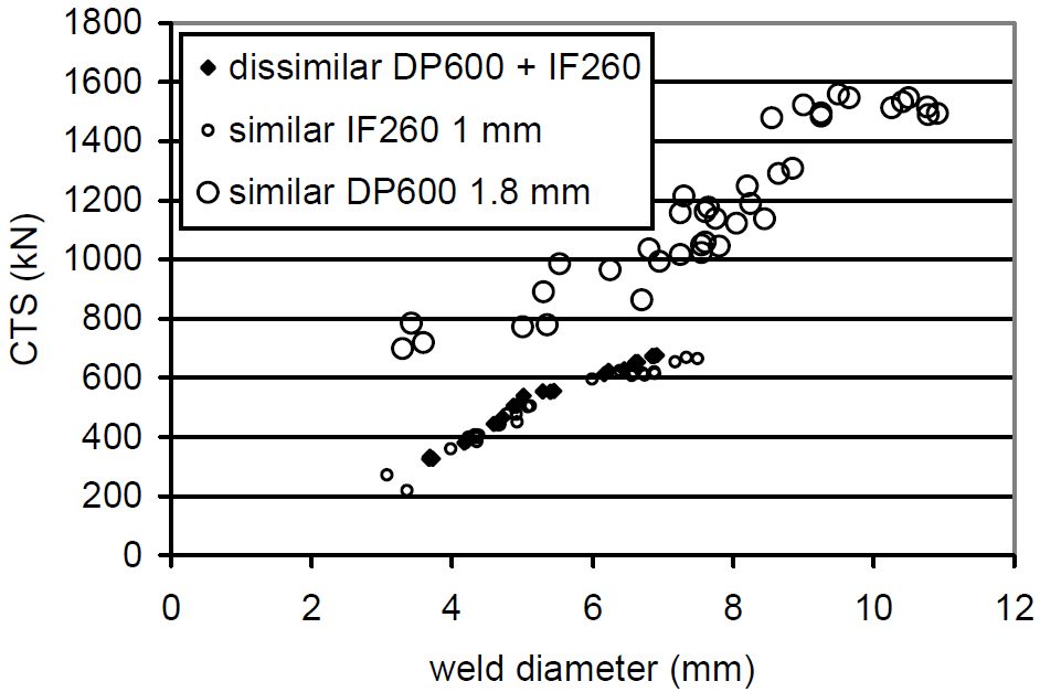
This study shows that the cross tension strength (CTS) is always higher than the strength expected from the lower strength material in the joint. Figure 1 verifies the assumption that the load bearing capacity of a heterogeneous configuration is supposed to equal the minimum strength of both homogenous assemblies. Material used in this study was a 1 mm low carbon equivalent Dual Phase 980 (DP980 LCE) steel.
Figure 1: Example of dissimilar configuration with CTS matching the “minimum rule”.B-6
The materials chosen for this study are in Table 1.
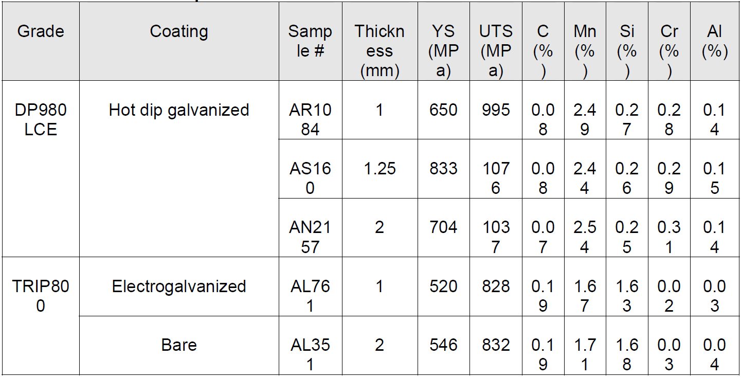
Table 1: Steel sheet samples.B-6
The material thickness combinations for all of the two sheet joints are shown in Table 2.
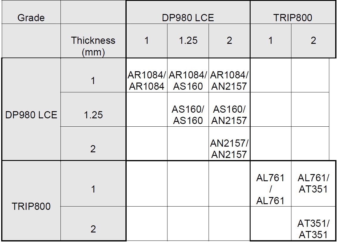
Table 2: Welded 2-sheet configurations.B-6
The three-sheet stackups all were made using the 1 mm DP980 LCE. These configurations were designed to understand what happens in such cases, knowing that three-sheet welding is very common in car body manufacturing. The three-sheet stackup configurations are shown in Figure 2 and are as were follows:
- a square DP980 coupon (patch) is inserted between the two classical cross-tension coupons for welding (1+patch+1 mm);
- two coupons oriented the same way welded with one coupon oriented in the transverse direction to form a cross-tension sample (1+[1+1] mm);
- same configuration as a) but the external coupon is removed by manual torsion before cross-tension testing (1+1+0 mm);
- same configuration as a), but the two coupons oriented the same way are first spot welded together strongly (with several spots) in the extremities, before the actual 3-sheet spot weld is done ([1++++1]+1 mm).
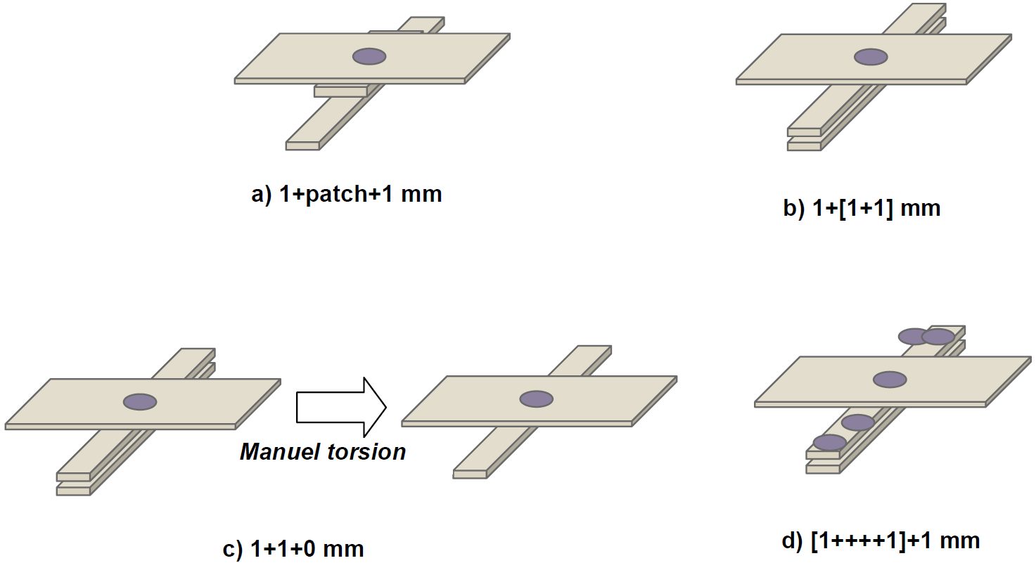
Figure 2: Three-sheet configurations based on 1mm DP980 LCE sample.B-6
The welding parameters for each configuration are listed in Table 3.
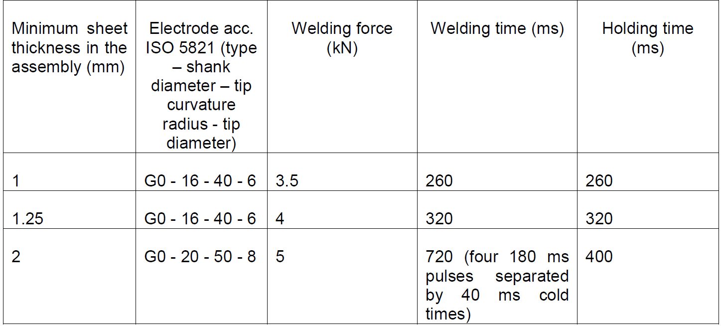
Table 3 : Welding parameters.B-6
CTS is strongly dependent on weld diameter (Figure 3).
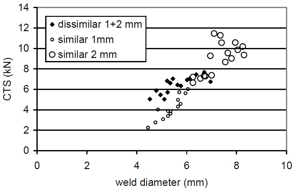
Figure 3: Cross-tension Strength for TRIP800 configurations.B-6
CTS for the main DP980 configurations are shown as a function of weld diameter in Figures 4 and 5.
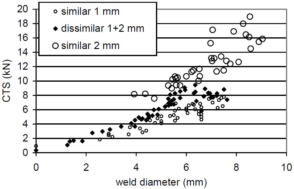
Figure 4: Cross-tension Strength for DP980 1+1, 1+2 and 2+2 configurations.B-6
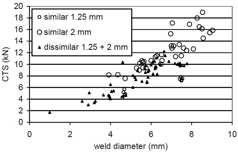
Figure 5: Cross-tension Strength for DP980 1.25+1.25, 1.25+2 and 2+2 configurations.B-6
The three-sheet configurations based on 1mm DP980 LC results are shown in Figures 6 and 7. These results again verify that dissimilar configuration performances appear above the “minimum rule” assumption described in Figure 1.
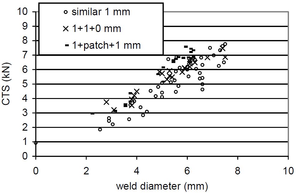
Figure 6: Cross-tension Strength for DP980 1+1, 1+1+0 and 1+patch+1 configurations.B-6
![Figure 7: Cross-tension Strength for DP980 1+1, 1+2, 1+[1+1]and [1+++1]+1 configurations.](https://ahssinsights.org/wp-content/uploads/2020/07/3114c_Fig7.jpg)
Figure 7: Cross-tension Strength for DP980 1+1, 1+2, 1+[1+1]and [1+++1]+1 configurations.B-6
The observation that CTS is greater than predicted by the “minimum rule” has been called a “positive deviation” from the expected strengths.
This work concluded that while material qualification tests are frequently based on similar welding configurations, real car body applications are quite systematically dissimilar configurations. For spot welds failing in plug mode, the strength of the assembly only depends on the weakest material strength. In case of AHSS+AHSS welded combinations, however, things turn out to be different. Similar grade but dissimilar thickness High-Strength Steel configurations have been spot welded and tested in Cross-Tension. The following main conclusions can be highlighted:
- For dissimilar thickness configurations, the cross-tensile strength is above the standard “minimum rule” assumptions, this phenomenon being called a “positive deviation”;
- Limited thermal and notch location effects can explain part of this positive deviation, but the main reason is mechanical;
- As evidenced through several analytic and numerical studies, this mechanical effect is due to the less severe local stresses at the notch in case of uneven thickness, and improves the positive deviation when the thickness ratio increases. Although widely used for material qualification and scientific purposes, similar configurations appear as the worst case in terms of cross-tension performance for high strength steels. Actual vehicle design should consider positive deviation in dissimilar configurations to maximize the potential strength of spot welds in High-Strength steels.
RSW of Dissimilar Steel
This article is the summary of a paper entitled, “HAZ Softening of RSW of 3T Dissimilar Steel Stack-up”, Y. Lu., et al.L-15
Electromechanical Model
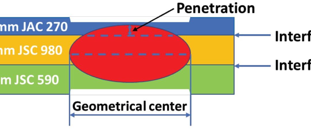
The study discusses the development of a 3D fully coupled thermo-electromechanical model for RSW of a three sheet (3T) stack-up of dissimilar steels. Figure 1 schematically shows the stack-up used in the study. The stack-up chosen is representative of the complex stack-ups used in BIW. Table 1 summarizes the nominal compositions of the three steels labeled in Figure 1.
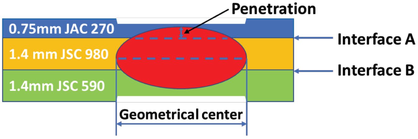
Figure 1: Schematics of the 3T stack-up of 0.75-mm-thick JAC 270/1.4-mm-thick JSC 980/1.4-mm-thick JSC 590 steels.L-15
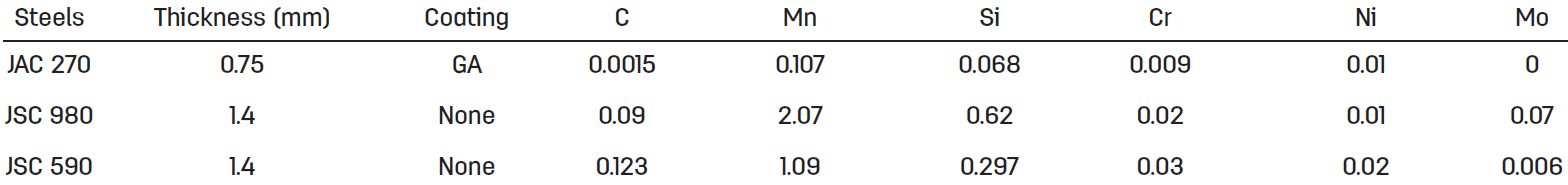
Table 1: Nominal Composition of Steels.L-15
JAC270 is a cold rolled Mild steel with a galvanneal coating having a minimum tensile strength of 270 MPa. JSC590 and JSC980 are bare cold rolled Dual Phase steels with a minimum tensile strength of 590 MPa and 980 MPa, respectively.
The electrodes used were CuZr dome-radius electrodes with a surface diameter of 6 mm. The welding parameters are listed in Table 2.
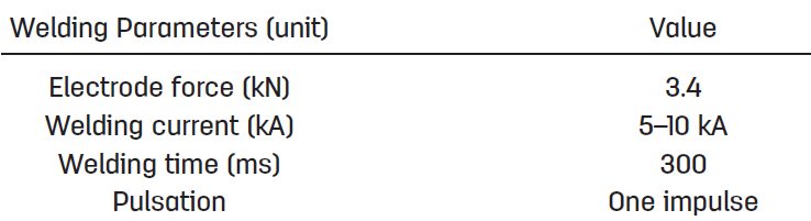
Table 2: Welding Parameters for Resistance Spot Welding of 3T Stack-Up of Steel Sheets.L-15
Figure 2 shows consistent nugget dimensions between simulation and experiment, supporting the validity of the RSW process model for 3T stack-up. The effect of welding current on nugget penetration into the thin sheet is similar to that on the nugget size. It increases rapidly at low welding current and saturates to 32% when the welding current is higher than 9 kA, as shown in Figure 2C.
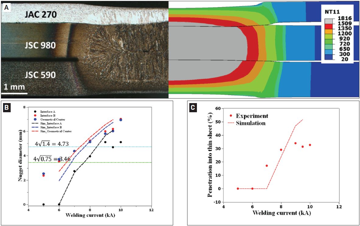
Figure 2: Comparison between experimental and simulated results: A) Nugget geometry at 8 kA; B) nugget diameters; C) nugget penetration into the thin sheet as a function of welding current. In Figure 2A, the simulated nugget geometry is represented by the distribution of peak temperature (in Celsius). The two horizontal lines in Figure 2B represent the minimal nugget diameter at Interfaces A and B calculated, according to AWS D8.1M: 2007, Specification for Automotive Weld Quality Resistance Spot Welding of Steel. Due to limited number of samples available for testing, the variability in nugget dimensions at each welding current was not measuredL-15.
The results for nugget formation during RSW of the 3T stack-up are show in Figures 3-5. Figure 2 shows that, at the start of welding, the contact pressure at interface A (thin/thick) has a higher peak and drops more quickly along the radial direction than that at interface B (thick/thick). Due to the more localized contact area (Figure 3), a high current density can be observed at interface A, as shown in Figure 4A. Additionally, due to the high current density at interface A, localized heating is generated at this interface, as shown in Figure 5A.
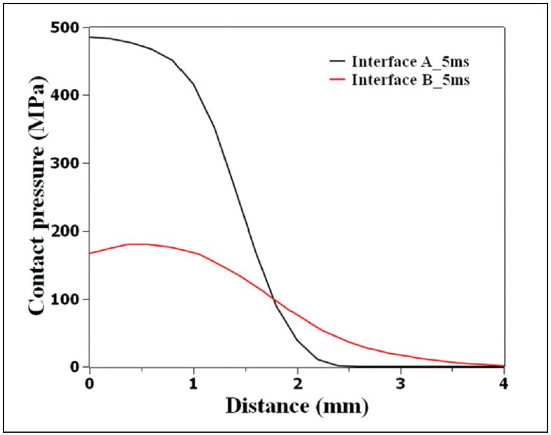
Figure 3: Calculated contact pressure distribution at interfaces A (thin/thick) and B (thick/thick) at a welding time of 5 ms, current of 8 kA, and electrode force of 3.4 L-15
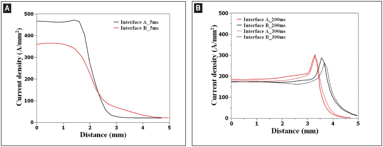
Figure 4: Calculated current density distribution at interfaces A (thin/thick) and B (thick/thick) at welding time of A — 5 ms; B — 200 and 300 ms.L-15
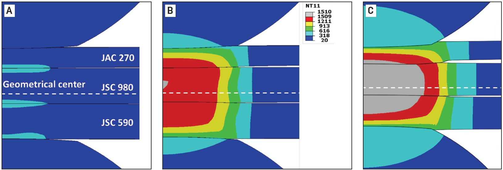
Figure 5: Temperature distribution during resistance spot welding of 3T stack-up at welding times of A) 5 ms; B) 102 ms; C) 300 ms. Welding current is 8 kA and electrode force is 3.4 kN. Calculated temperature is given in Celsius.L-15
As welding time increases, the contact area is expanded, resulting in a decrease of current density. The heat generation rate is shifted from interfaces to the bulk and the peak temperature occurs near the geometrical center of the stack-up.
Figure 6 illustrates that the predicted value corresponds well with the experimental data indicating a sound fitting to the isothermal tempering experimental data.
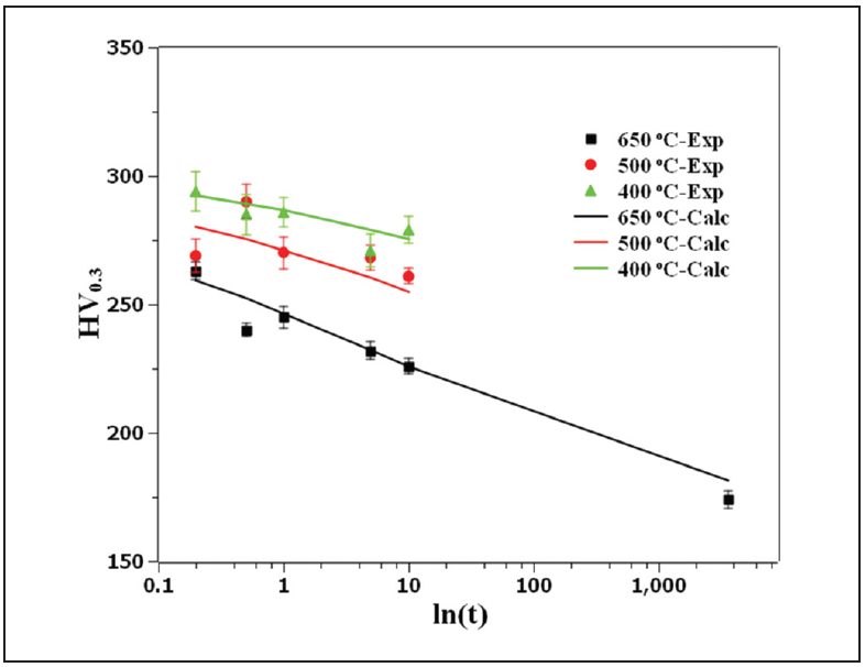
Figure 6: Comparison of the measured hardness with JMAK calculation showing the goodness of fit of the JSC 980 tempering kinetics parameters.L-15
Figure 7 shows the predicted hardness map of RSW 3T stack-up as well as the predicted and measured hardness profiles for JSC 980.
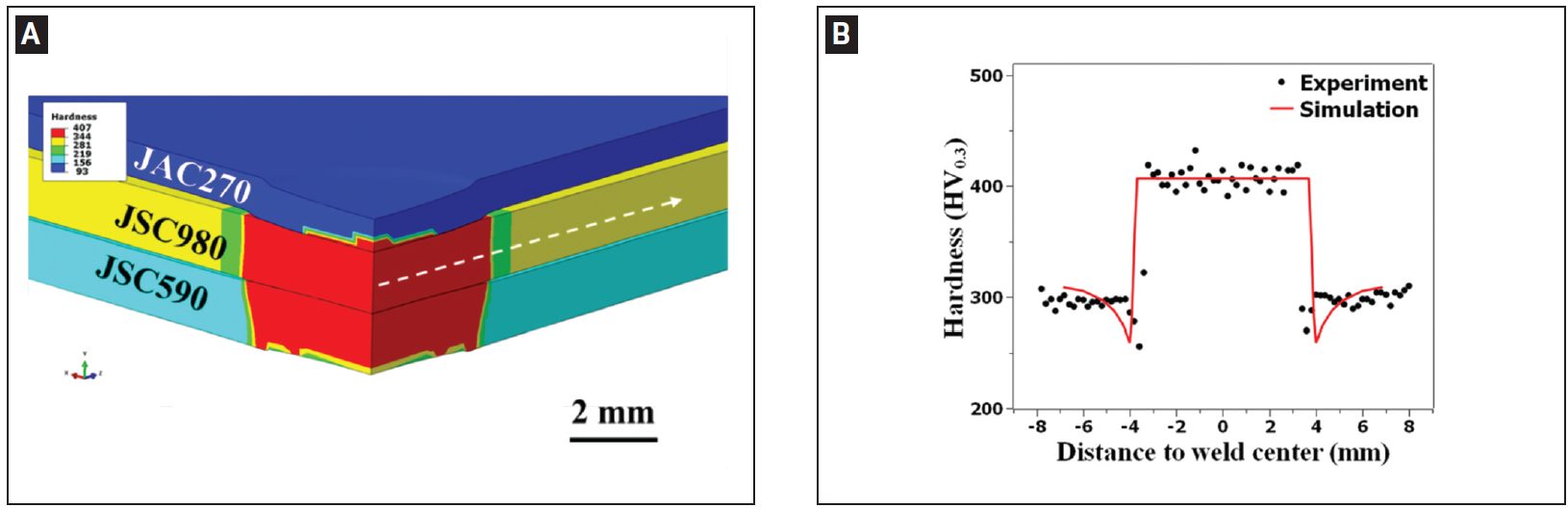
Figure 7: A) Predicted hardness map of resistance spot welded 3T stack-up; B) predicted and measured hardness profiles along the line marked in (A) for JSC 980.L-15
Automotive Welding Process Comparison
Introduction
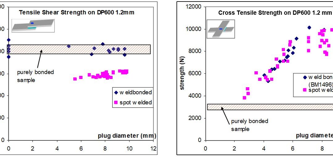
A solution to improve the spot weld strength is to add a HS adhesive to the weld. Figure 1 illustrates the strength improvement obtained in static conditions when crash adhesive (example: Betamate 1496 Dow Automotive) is added. The trials are performed with 45-mm-wide and 16-mm adhesive bead samples.
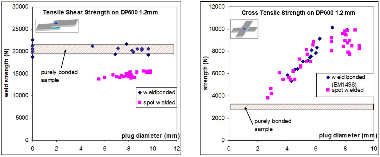
Figure 1: TSS and CTS on DP 600.A-16
Another approach to improve the strength of welds is done by using laser welding instead of spot welding. The technologies based on remote welding optics have been introduced and a high productivity can be obtained. The effective welding time is maximized and a wide variety of weld geometries becomes feasible. Compared to spot welding, the main advantage of laser welding, regarding mechanical properties of the joint, is the possibility to adjust the weld dimension to the requirement. One may assume that, in tensile shear conditions, the weld strength depends linearly of the weld length (Figure 2).
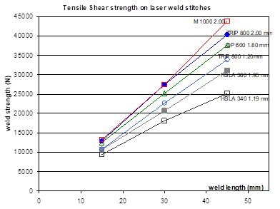
Figure 2: Tensile-shear strength on laser weld stitches of different length.A-16
Comparing spot weld strength with laser weld strength cannot be restricted to the basic tensile shear test. Tests were performed to evaluate the weld strength in both quasi-static and dynamic conditions under different solicitations, on various UHSS combinations. The trials were performed on a high-speed testing machine, at 5 mm/min for the quasi-static tests and 0.5 m/s for the dynamic tests (pure shear, pure tear or mixed solicitation) (Figure 3). The strength at failure and the energy absorbed during the trial have been measured. It should be noticed that the energy absorbed depends also on the deformation of the sample. However, as all the trials were made according to the same sample geometry, the comparison of the results is relevant. Laser stitches were done with a 27-mm length. C- and S-shape welds were performed with the same overall weld length. This lead s to various apparent length and width of the welds. A shape factor, expressed as the ratio width/length of the weld, can be defined according to Table 1.
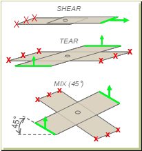
Figure 3: Sample geometry for quasi-static and dynamic tests. A-16
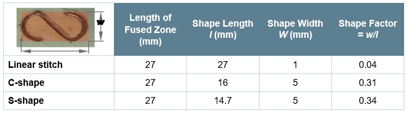
Table 1: Shape factor definition.A-16
The weld strength at failure can be easily described with an elliptic representation, with major axes representing pure shear and normal solicitation (Figure 4). For a reference spot weld corresponding to the upper limit of the weldability range, globally similar weld properties can be obtained with 27-mm laser welds. The spot weld equivalent length of 25-30 mm has been confirmed on other test cases on UHSS in the 1.5- to 2-mm range thickness. It has also been noticed that the spot weld equivalent length is shorter on thin mild steel (approximately 15-20 mm). This must be considered in case of shifting from spot to laser welding on a given structure. There is no major strain rate influence on the weld strength; the same order of magnitude is obtained in quasi-static and dynamic conditions.
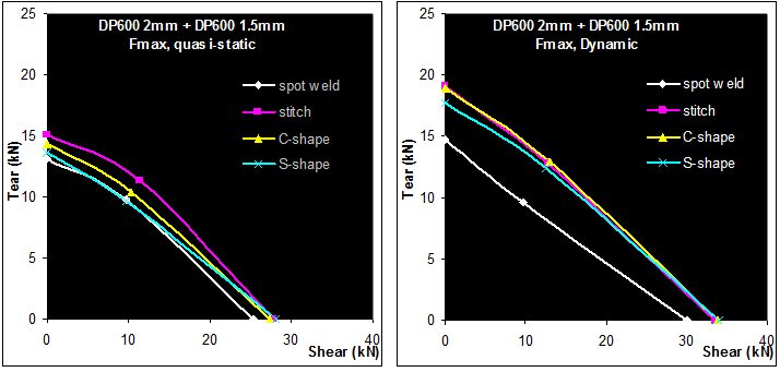
Figure 4: Quasi-static and dynamic strength of welds, DP 600 2 mm+1.5 mm.A-16
The results in terms of energy absorbed by the sample are seen in Figure 5. In tearing conditions, both the strength at fracture and energy are lower for the spot weld than for the various laser welding procedures. In shear conditions, the strength at fracture is equivalent for all the welding processes. However, the energy absorption is more favorable to spot welds. This is due to the different fracture modes of the welds. IF fracture is observed on the laser welds under shearing solicitation (Figure 6). Even if the strength at failure is as high as for the spot weds, this brutal failure mode leads to lower total energy absorption.
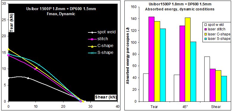
Figure 5: Strength at fracture and energy absorption of HF1500P 1.8-mm + DP 600 1.5-mm samples for various welding conditions. A-16
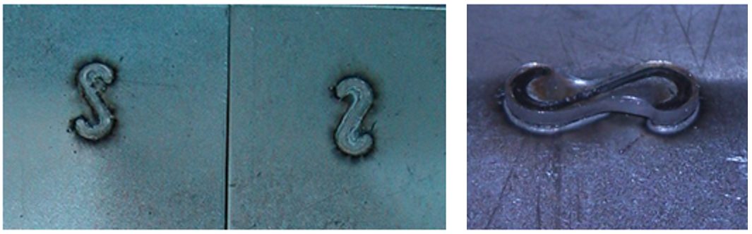
Figure 6: IF fracture mode (left), “plug-out” fracture mode (right).A-16
Figure 7 represents the energy absorbed by omega-shaped structures and the corresponding number of welds that fail during the frontal crash test (here on TRIP 800 grade). It appears clearly that laser stitches have the highest rate of fracture during the crash test (33%). In standard spot welding, some weld fractures also occur. It is known that UHSS are more prone to partial IF fracture on coupons, and some welds fail as well during the crash test. By using either Weld-Bonding or adapted laser welding shape, there is no more weld fractures during the test, even if the parts are severely crashed and deformed. As a consequence, higher energy absorption is also observed.
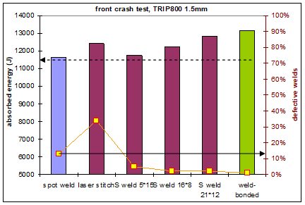
Figure 7: Welding process and weld shape influence on the energy absorption and weld integrity on frontal crash tests. A-16
Regarding stiffness, up to 20% improvement can be obtained. The best results are obtained with continuous joints, and particularly using adhesives. Adhesive bonding and weld- bonding lead to the same results of the stiffness improvement only being due to the adhesive, not to the additional welds.
Figure 8 shows the evolution of the torsional stiffness with the joining process.
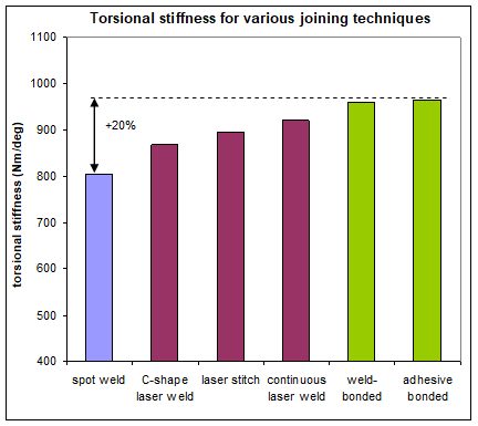
Figure 8: Evolution of the torsional stiffness with the joining process.A-16
Optimized laser joining design leads to same performances as a weld bonded sample regarding fracture modes seen in Figure 9.
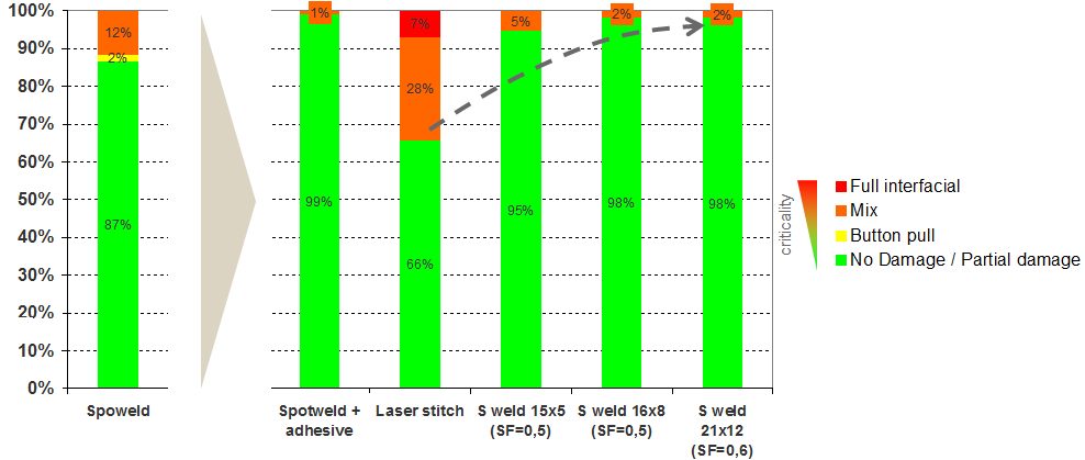
Figure 9: Validation test case 1.2-mmTRIP 800/1.2-mm hat-shaped TRIP 800.
Top-hat crash boxes were tested across a range of AHSS materials including DP 1000. The spot weld’s energy absorbed increased linearly with increasing material strength. The adhesives were not suitable for crash applications as the adhesive peels open along the entire length of the joint. The welded bond samples perform much better than conventional spot welds. Across the entire range of materials there was a 20-30% increase in mean force when WB was used. The implications of such a large increase in crash performance are very significant. The results show that when a 600 MPa steel is weld bonded it can achieve the same crash performance as a 1000 MPa steel in spot-welded condition. It is also possible that some down gauging of materials could be achieved, but as the strength of the crash structure is highly dependent upon sheet thickness only small gage reductions would be possible.
Figure 10 shows the crash results for spot-welded and weld-bonded AHSS.
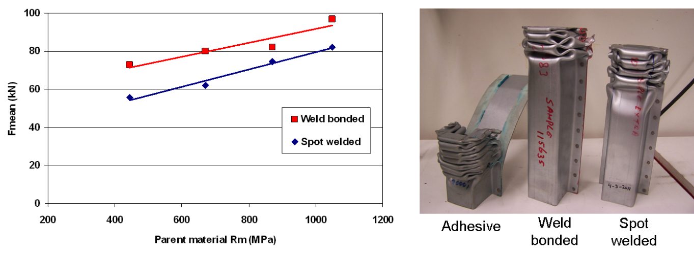
Figure 10: Crash results for spot-welded and weld-bonded AHSS.
There are numerous welding processes available for the welding of AHSS in automotive applications. Each of these processes has advantages and disadvantages that make them more or less applicable for particular applications. These qualities include joint efficiency, joint fit-up and design, joint strength, and stiffness, fracture mode, and cost effectiveness (equipment cost, production rates, etc.). The following data can allow for comparisons to be made for automotive application welding and joining processes, as well as possible repair substitutions.
Many tests were performed using lap and coach joints, reduced specimen overlap distance, and adjusted weld sizes to more closely represent typical joints consistent with automotive industry acceptance criteria. The tests were aimed at providing a baseline reference for a wide variety of welding and joining processes and material combinations. In general, there was no correlation between joint efficiency, normalized energy, and normalized stiffness. Joint efficiency was calculated by dividing the peak load of the joint by the peak load of the parent metal. Some processes, joint configurations and material combinations have high joint efficiency and energy, while others result in high joint efficiency but low energy. Few processes showed high values for all metrics across all materials and joint configurations (Figure 11). It was observed that peak loads tended to increase, on average, as material strength increased for lap joints (Figure 12). However, joint efficiency generally decreased as material strength increased. Therefore, joint strength did not increase in proportion to parent material strength increase for most of the processes and materials studied. Coach joints generally showed lower joint efficiency and stiffness than lap joints (Figure 13). Process and material combinations should be selected based on the required performance, joint design, and cost.A-12
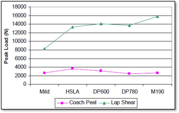
Figure 11: Average peak loads (all processes combined).A-12
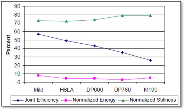
Figure 12: Lap shear average joint efficiency, normalized energy and stiffness (all processes combined).A-12
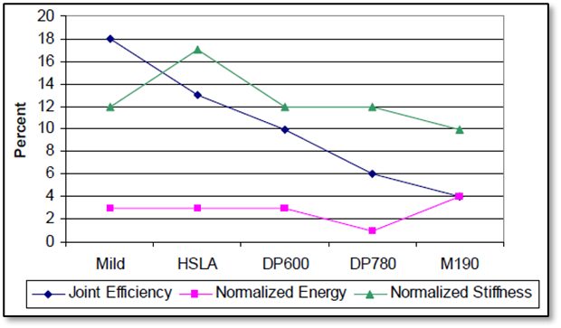
Figure 13: Coach peel average joint efficiency, normalized energy and stiffness (all processes combined).A-12
All Processes General Comparison
Numerous tests were performed using the most popular automotive joining processes including RSW, GMAW/brazing, laser welding/brazing, mechanical fasteners, and adhesive bonding. Joint efficiency and normalized energy of all the processes were compared for HSLA steels, DP 600 samples, DP 780 samples, and M190 samples. Joint efficiency was calculated as the peak load of the joint divided by the peak load of the parent metal. Energy was calculated as the area under the load/displacement curve up to peak load.
The materials used consisted of 1.2-mm EG HSLA, 1.2-mm galvanized DP 600, 1.0-mm GA DP 780, and 1.0-mm EG M190. The testing configuration matrix (Table 2) lists the materials and process combinations studied. The tolerance of weld lengths is ±10%. Lap-shear joints were centered in the overlap for all processes except lap fillet welds and brazes. Coach-peel joints were centered in the overlap for all processes (Figure 14). A-12
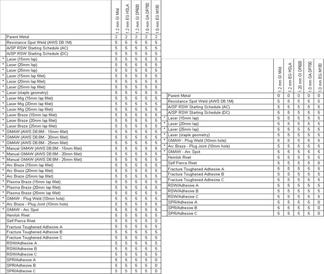
Table 2: Lap-shear (left) and coach-peel (right) test configuration matrix.A-12
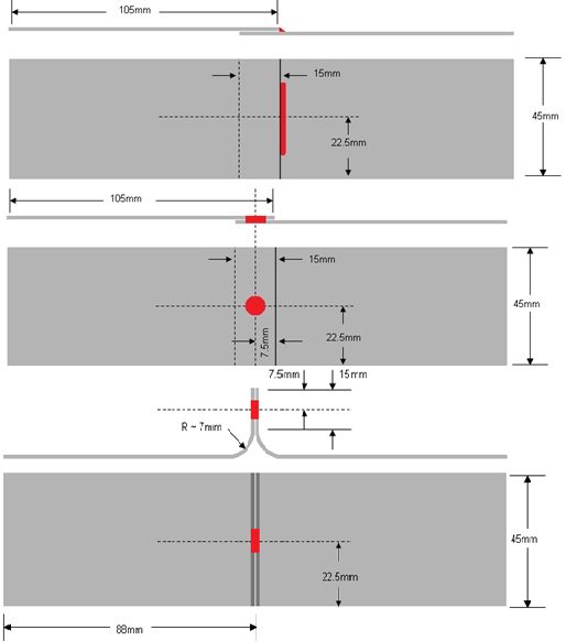
Figure 14: Lap-shear and coach-peel set-up.A-12
DP 600 samples, DP 780 samples, and M190 samples. Joint efficiency was calculated as the peak load of the joint divided by the peak load of the parent metal. Energy was calculated as the area under the load/displacement curve up to peak load.
Self-piercing riveting with adhesive gave the greatest overall joint efficiency for the HSLA lap shear tests, while laser obtained the largest normalized energy (Figure 15a and 15b).
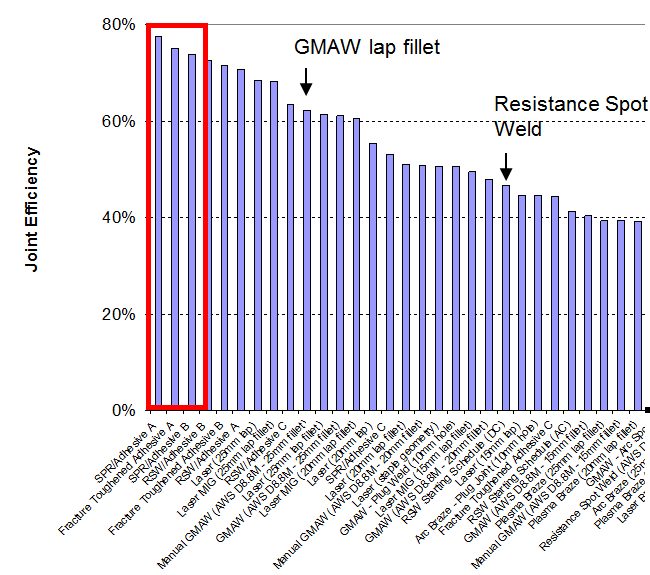
Figure 15a: Joint efficiency of HSLA lap-shear tests for all processes.A-12
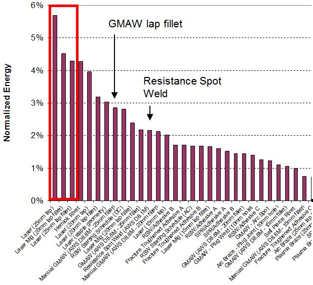
Figure 15b: Normalized energy of HSLA lap-shear tests for all processes.A-12
Self-penetrating riveting with adhesive gave the greatest overall values for both joint efficiency and normalized energy for lap shear testing of DP 600 samples (Figure 16a and 16b). However, coach peel testing of DP 600 obtained the best results with laser welding (Figure 17).
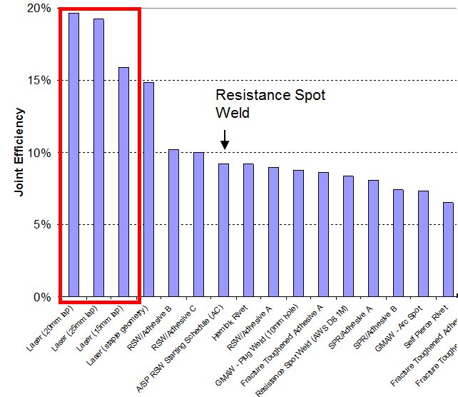
Figure 17a: Joint efficiency of DP 600 lap shear for all processes.A-12
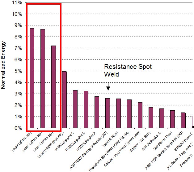
Figure 16b: Normalized energy of DP 600 lap shear for all processes.A-12
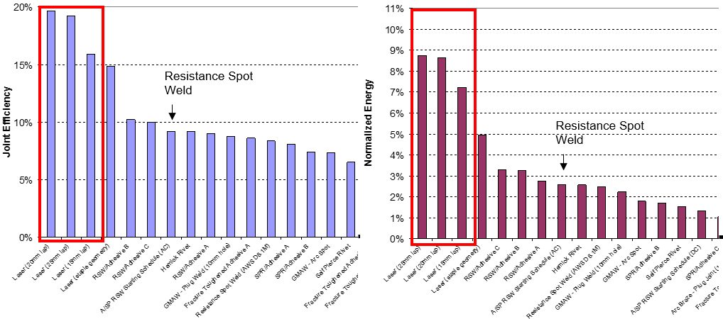
Figure 17: Joint efficiency and normalized energy of DP 600 coach peel for all processes.A-12
For the DP 780 lap-shear test, the best results out of all the tested processes were from laser/MIG welding, leading in both joint efficiency and normalized energy (Figure 18). Full laser welding produced the best results for coach-peel tests of the DP 780 samples (Figure 19).
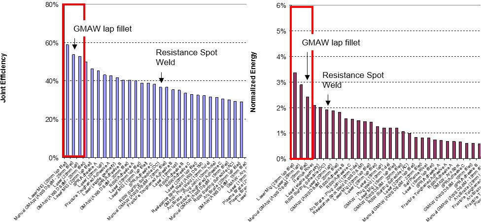
Figure 18: Joint efficiency and normalized energy of DP 780 lap shear for all processes.A-12
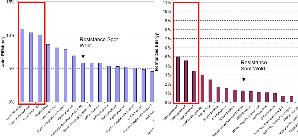
Figure 19: Joint efficiency and normalized energy of DP 780 coach peel for all processes.A-12
The M190 lap-shear samples had the best joint efficiency using RSW with adhesive, but full laser welding gave better normalized energy (Figure 20). The coach peel tests also had the best normalized energy with full laser welding. The best joint efficiency of the coach peel tests was produced from laser welding with staples (Figure 21).
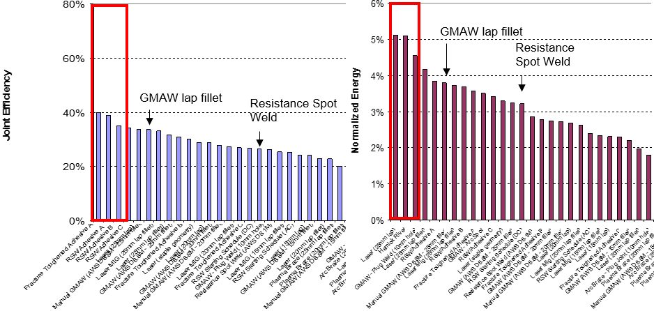
Figure 20: Joint efficiency and normalized energy of M190 lap shear for all processes.A-12
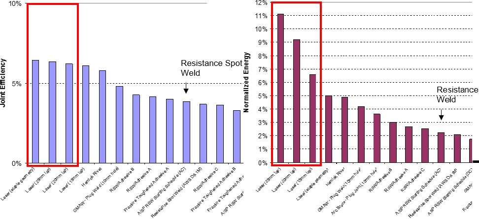
Figure 21: Joint efficiency and normalized energy of M190 coach peel for all processes.A-12
Cost Effectiveness Comparison: Spot Welding to Spot/Laser Welding Mixture
When automotive manufacturers are weighing the advantages and disadvantages of RSW to those of a spot/laser welding mixture process, cost effectiveness is a major concern. Spot/laser mixture welding has 38% lower operation cost compared to full spot welding because the laser installation performs more welds than a spot welding robot. Also, there are fewer robots to maintain and less consumables. The global cost is similar, but the spot/laser solution is about 4% less expensive overall. Figure 22 shows a cost comparison of spot welding and spot/laser welding.
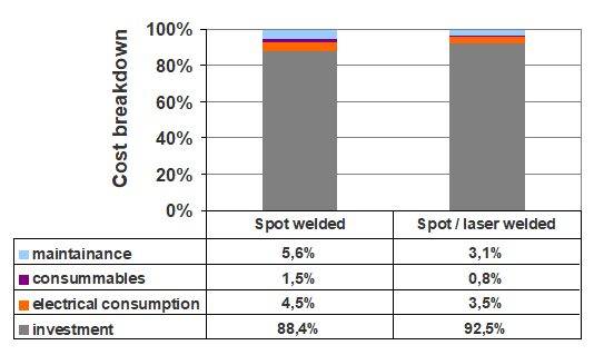
Figure 22: Cost comparison of spot welding and spot/laser welding.A-16
GMAW Compared to Laser Welding
When comparing the advantages and disadvantages of GMAW to those of laser welding in automotive applications, joint efficiency is a key subject. Numerous welds were made using both processes on 15- and 25-mm-thick pieces of materials varying in strength. All results showed that laser welding continuously had greater joint efficiency than GMAW (Figure 23).
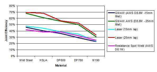
Figure 23: Joint efficiency of GMAW and laser welding for various steel strengths.
Back To Top
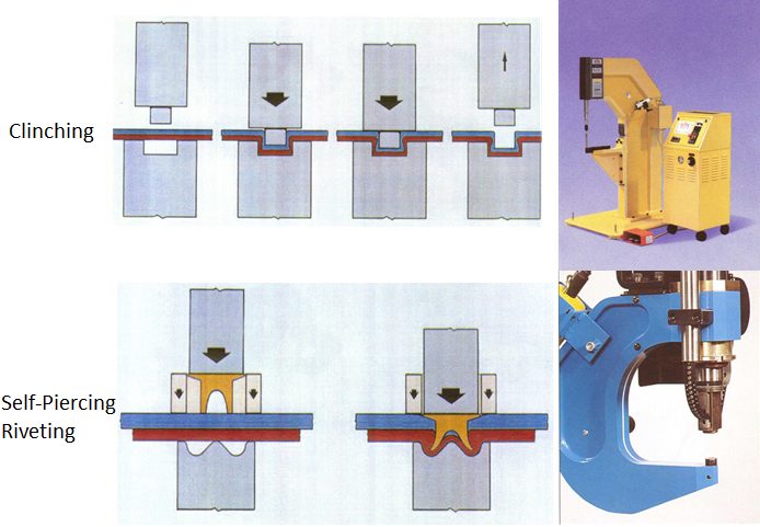
Mechanical Joining
Examples of mechanical joining in automotive manufacturing are clinching and self-piercing riveting. The process steps and typical equipment for both processes are shown in Figure 1. A simple round punch presses the materials to be joined into the die cavity. As the force continues to increase, the punch side material is forced to spread outward within the die side material.
Figure 1: Process steps and equipment for mechanical joining in automotive industries.
This creates an aesthetically round button, which joins cleanly without any burrs or sharp edges that can corrode. Even with galvanized or aluminized sheet metals, the anti-corrosive properties remain intact as the protective layer flows with the material. Table 1 shows characteristics of different mechanical joining methods.
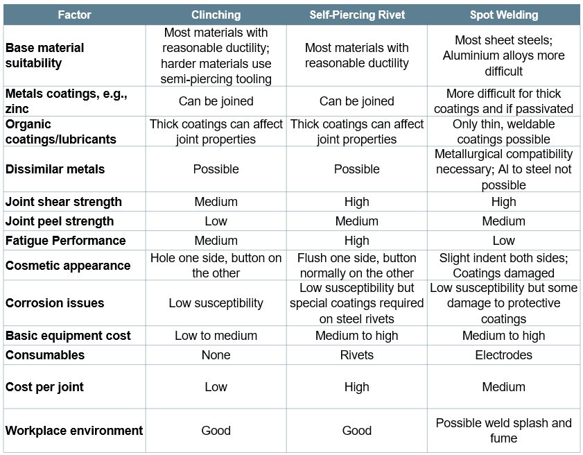
Table 1: Characteristics of mechanical joining systems.T-12
In a recent study conducted to assess the feasibility of clinch joining advanced HSST-8, it was concluded that 780-MPa DP and TRIP [link to steel material grades] steels can be joined to themselves and to low-carbon steel (see Figure 2). However, 980 DP steel showed tears when placed on the die side (Figure 3). These cracks were found at the ferrite- martensite boundaries (Figure 4). However, these tears did not appear to affect the joint strength. More work is needed to improve the local formability of 980 MPa tensile strength DP steel for successful clinch joining.
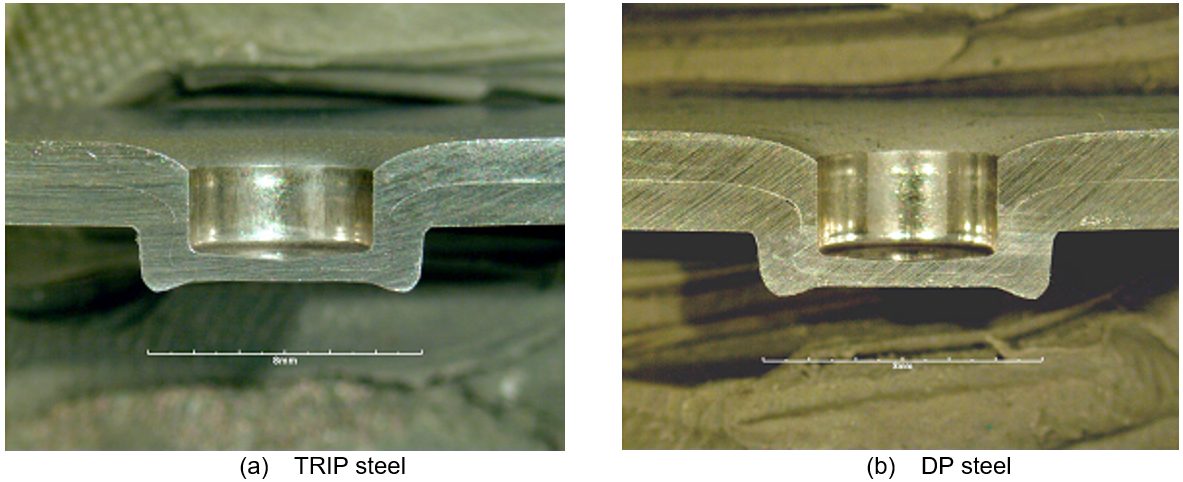
Figure 2: Cross sections of successful clinch joints in 780-MPa tensile.
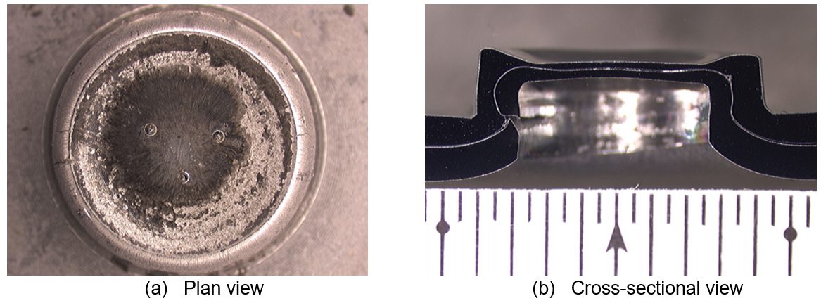
Figure 3: Clinch joint from DP 980-MPa steel showing tears on the die side.
Figure 4: SEM views of tears found in DP 980-MPa steel clinch joints.
Circular clinching without cutting and self-piercing riveting (existing half-hollow-rivets) are not recommended for materials with less than 40% hole expansion ratio (λ) as shown in Figure 5. Clinching with partial cutting may be applied instead.
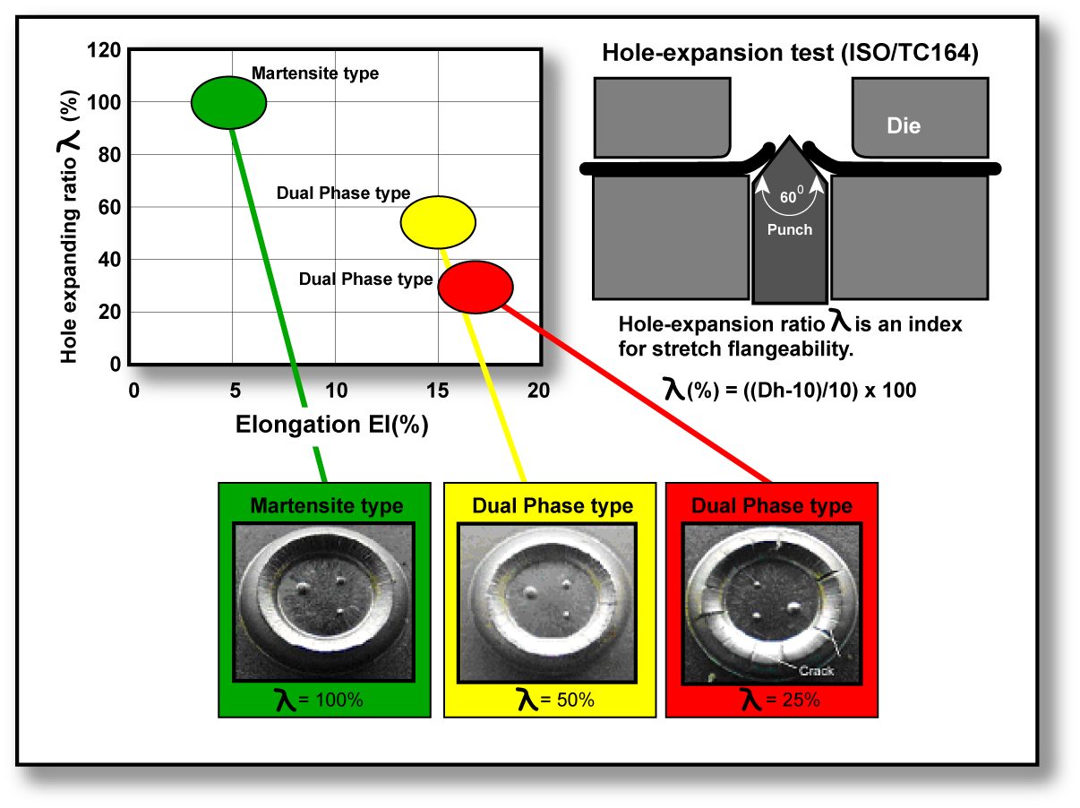
Figure 5: Balance between elongation and stretch flangeability of 980-MPa tensile-strength class AHSS and surface appearance of mechanical joint at the back side.N-1
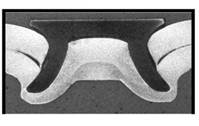
Figure 6: Example of DP 300/500 with a self-piercing rivet.G-2
Warm clinching and riveting are under investigation for material with less than 12T total elongation. As with any steel, equipment size and clinch/pierce force are proportional to the material strength and tool life is inversely proportional to material strength.
The strength of self-piercing riveted AHSS is higher than for mild steels. Figure 4.P-6 shows an example of a self-piercing rivet joining two sheets of 1.5-mm-thick DP 300/500. AHSS with tensile strengths greater than 900 MPa cannot be self-piercing riveted by conventional methods today.
Self-piercing rivet joints are typically similar or slightly weaker in strength when compared to spot welds. It is largely dependent on the punch-die size, design, and rivet size. However, self-piercing rivets usually perform better in fatigue loading compared to spot welds because there is no notch effect such as what exists in spot-welded joints Figure 7 (left)]. Although clinch joining is being used in several automotive applications, their performance is lower as shown in Figure 7 (right). Thus, they are not recommended for critical joints in automotive manufacturing.
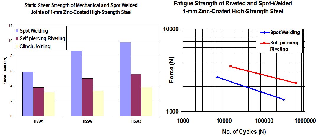
Figure 7: Strength performance for various mechanical joining methods.
Hybrid Riveting Adhesive
Self-piercing rivets can also be combined with adhesives to result in increased initial stiffness, YS, failure loads and fatigue strength when compared to spot welds using adhesives (Figure 8).
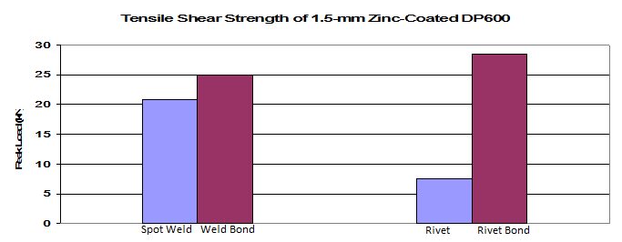
Figure 8: Tensile shear strength of SPR with adhesives and RSW with adhesives.
Arc Welding
Gas Metal Arc Welding: Introduction
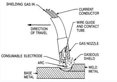
Gas Metal Arc Welding (GMAW) (Figure 1), commonly referred to by its slang name “MIG” (metal inert gas welding) uses a continuously fed bare wire electrode through a nozzle that delivers a proper flow of shielding gas to protect the molten and hot metal as it cools. Because the wire is fed automatically by a wire feed system, GMAW is one of the arc welding processes considered to be semi-automatic. The wire feeder pushes the electrode through the welding torch where it makes electrical contact with the contact tube, which delivers the electrical power from the power supply and through the cable to the electrode. The process requires much less welding skill than Shielded Metal Arc Welding (SMAW) or Gas Tungsten Arc Welding (GTAW) [LINK TO SECTION] and produces higher deposition rates.
Figure 1: GMAW
The basic equipment components are the welding gun and cable assembly, electrode feed unit, power supply, and source of shielding gas. This set up includes a water-cooling system for the welding gun which is typically necessary when welding with high duty cycles and high current.
GMAW became commercially available in the late 1940s offering a significant improvement in deposition rates and making welding more efficient. Deposition rates are much higher than for SMAW and GTAW, and the process is readily adaptable to robotic applications. Because of the fast welding speeds and ability to adapt to automation, it is widely used by automotive and heavy equipment manufacturers, as well as a wide variety of construction and structural welding, pipe and pressure vessel welding, and cladding applications. It is extremely flexible and can be used to weld virtually all metals. Relative to SMAW, GMAW equipment is a bit more expensive due to the additional wire feed mechanism, more complex torch, and the need for shielding gas, but overall it is still relatively inexpensive.
GMAW is “self-regulating”, which refers to the ability of the machine to maintain a constant arc length at all times. This is usually achieved using a constant-voltage power supply, although some modern machines are now capable of achieving self-regulation in other ways. This self-regulation feature results in a process that is ideal for mechanized and robotic applications.
Figure 2 provides important GMAW terminology. Of particular importance is electrode extension. As shown, electrode extension refers to the length of filler wire between the arc and the end of the contact tip. The reason for the importance of electrode extension is that the longer the electrode extension, the greater the amount of resistive (known as I2R) heating that will occur in the wire. Resistive heating occurs because the steel wire is not a good conductor of electricity. This effect can become significant at high currents and/or long extensions, and can result in more of the energy from the power supply being consumed in the heating and melting of the wire, and less in generating arc heating. As a result, significant resistive heating can result in a wider weld profile with less penetration or depth of fusion. The stand-off distance is also an important consideration. Distances that are excessive will adversely affect the ability of the shielding gas to protect the weld. Distances that are too close may result in excessive spatter build-up on the nozzle and contact tip. Various gases are being used for shielding the in GMAW process. The most common ones include argon (Ar), helium (He), and carbon dioxide (CO2) and combinations of these. Figure 3 illustrates the effect of the shielding gas on the weld profile.
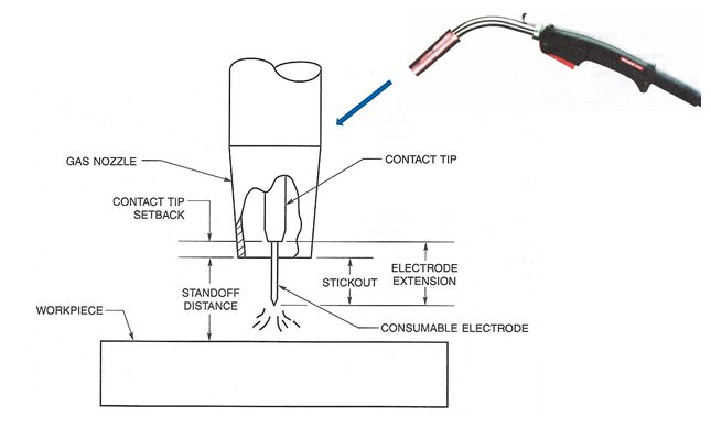
Figure 2: Common GMAW terminology
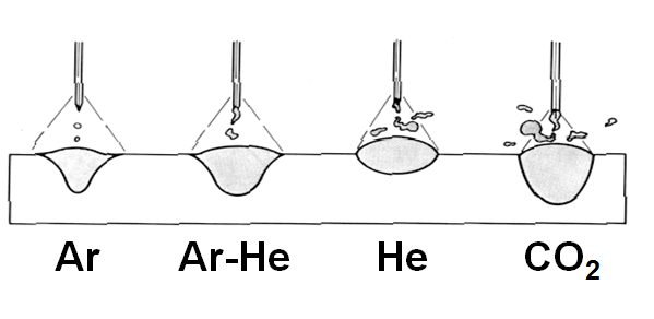
Figure 3: Effect of shielding gas on weld profile
AWS A5.18 is the carbon steel filler metal specification for SMAW, and includes both filler metal for both GMAW and GTAW. A typical electrode is shown on Figure 4. The “E” refers to electrode and the “R” refers to rod which means the filler metal can be used either as a GMAW electrode which carries the current, or as a separate filler metal in the form of a rod that could be used for the GTAW process. The “S” distinguishes this filler metal as solid (vs. the “T” designation which refers to a tubular GCAW electrode or “C” for composite electrode), the number, letter, or number/letter combination which follows the S refers to a variety of information about the filler metal such as composition, recommended shielding gas, and/or polarity.
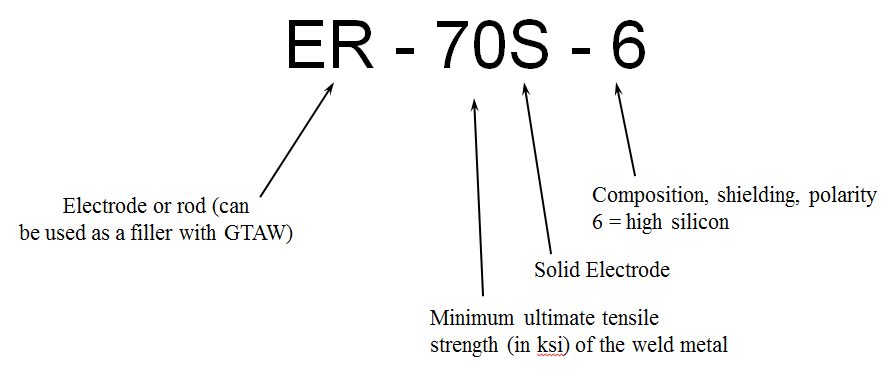
Figure 4: Typical AWS A5.18 electrode.
In summary, the GMAW process offers the following advantages and limitations:
- Advantages:
- Higher deposition rates than SMAW and GTAW
- Better production efficiency vs. SMAW and GTAW since the electrode or filler wire does need to be continuously replaced
- Since no flux is used there is minimal post-weld cleaning required and no possibility for a slag inclusion
- Requires less welder skill than manual processes
- Easily automated
- Can weld most commercial alloys
- Deep penetration with spray transfer mode
- Depending on the metal transfer mode, all position welding is possible
- Limitations:
- Equipment is more expensive and less portable than SMAW equipment
- Torch is heavy and bulky so joint access might be a problem
- Various metal transfer modes add complexity and limitations
- Susceptible to drafty conditions
GMAW Procedures and Properties
Despite the increase alloying content used for Q&P 980, there is no increased welding defect type or rate compared with mild steel Gas Metal Arc Welding (GMAW) welds. Figure 5 is the microhardness profile of 1.6-mm Q&P 980’s GMAW weld joint. Both welded seam and HAZ are all less than 500 HV, and there is no obvious softened zone in HAZ.B-4
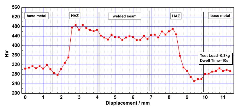
Figure 5: Microhardness profile of 1.6-mm DP 980’s GMAW weld joint. B-4
GMAW was used on three steels studied under a range of conditions. The left represents the FZ location and the middle is the HAZ. The figures show various degrees of HAZ hardening and softening depending on material grade and other conditions. The highest hardness occurs in the near HAZ, while the softest point is in the far HAZ. DP 980 [LINK TO THE MATERIAL IN METALLURGY] shows the greatest degree of HAZ hardening and softening. The nominally high CR condition is a combination of low heat input and heat sink. The plots show that CR tends to have the largest effect on the DP steels, with the TRIP steel being somewhat less affected. Pre-strain has the largest effect on the TRIP Base Metal (BM) , increasing the BM hardness by about 25%. The hardness of the softest location of the TRIP 780 HAZ is also increased by pre-strain, although degree of softening (about 20%) is not significantly changed. Pre-straining increased the DP 780 BM hardness by only about 10%. Pre-straining did not affect the peak HAZ hardness for either material. Post-baking did not appear to have a significant influence on the HAZ hardness profiles of the DP 780 material or the TRIP 780 material, regardless of pre-strain condition (Figures 6 through 8).
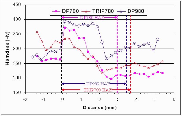
Figure 6: Hardness profiles of DP 780, TRIP 780, and DP 980 lap welds produced with the nominally high CR, no pre-strain or post-baking.P-7

Figure 7: Hardness profiles of DP 780 and TRIP 780 welds
produced both with and without pre-strain for the high CR condition.E-1
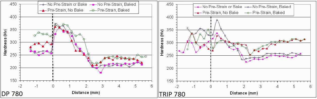
Figure 8: Hardness profiles of DP 780 and TRIP 780 welds produced both
with and without post-baking for both pre-strained sheet and not pre-strained
sheet for the nominally high CR condition.E-1
TRIP 780 lap joint static tensile results for different filler metal and CR conditions are shown in Figure 9. The results are expressed in terms of joint efficiency and the strain at peak load. The data indicates joint efficiencies ranged from about 50% to about 98%. Strains at peak load ranged from less than 3% to nearly 8%. Fracture occurred either in the far HAZ or at the weld fusion boundary. Filler metal strength had no discernable effect on the tensile properties. Figure 9 shows static tensile test results of the TRIP 780 butt joints. All the welds failed in the softened region of the far HAZ with joint efficiencies in excess of 89%. On average, welds made using higher CR experienced higher strains during loading than those made using lower CR. As was the case with the lap welds, filler metal strength did not appear to influence the static tensile properties. The abbreviations of high and low “CR” indicate high and low CR used for each weld.
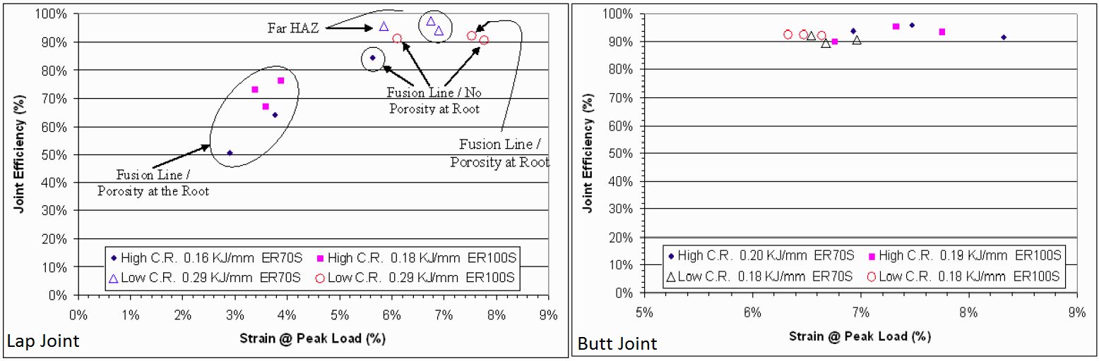
Figure 9: Static tensile test results of TRIP 780 lap and butt joints.E-1
The static tensile test results of the DP 780 butt welds are shown in Figure 10. All welds failed in the softened region of the far HAZ. As shown, the high CR welds had joint efficiencies in excess of 90%. The high CR welds also appear to have slightly greater strains at peak load.
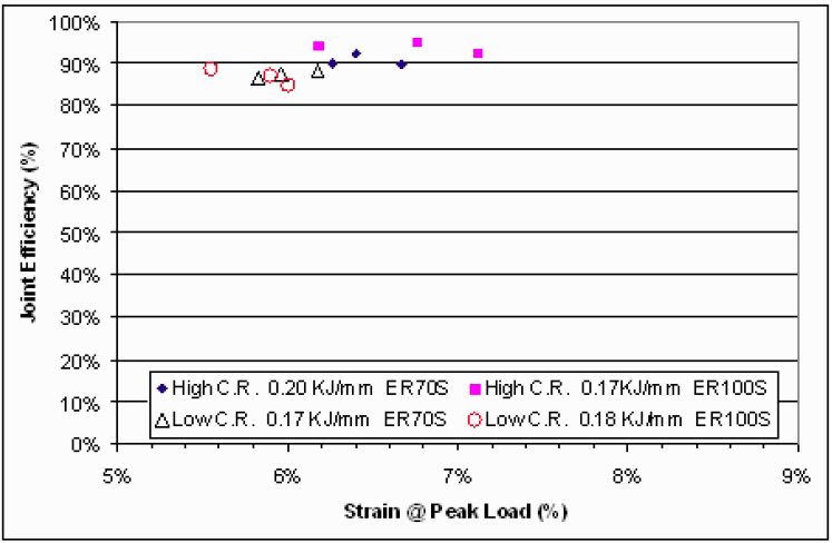
Figure 10: Static tensile test results of DP 780 butt joints.E-1
Figure 11 (left) shows the TRIP 780 lap joint dynamic tensile results for different filler metal and CR conditions. UTS ranged from 372 to 867 MPa (54 to 126 ksi) and strain at peak load ranged from less than 1% to over 5%. The high CR lap joints had lower strengths and strains at peak load. These welds failed along the fusion line presumably due to porosity present at the root. All the low CR lap welds produced with the ER70S-6 wire failed in far HAZ of the bottom sheet. Of the low CR lap joints produced with the ER100S-G wire, two dynamic tensile specimens failed in the softened region of the far HAZ, and one failed along the fusion line of the top sheet without the presence of porosity at the weld root. Analysis of Figure 11 (left) indicates that filler metal strength did not have a distinguishable effect on the dynamic tensile test results. Figure 11 (right) shows the dynamic tensile test results of the TRIP 780 butt joints. All failed in the softened region of the far HAZ. The UTS of the butt joints ranged from 840 to 896 MPa (122 to 130 ksi), and strain at peak load was generally between 3 and 4%. The figure indicates that neither filler metal strength nor CR condition had a distinguishable effect on the dynamic tensile test results of the butt joints.
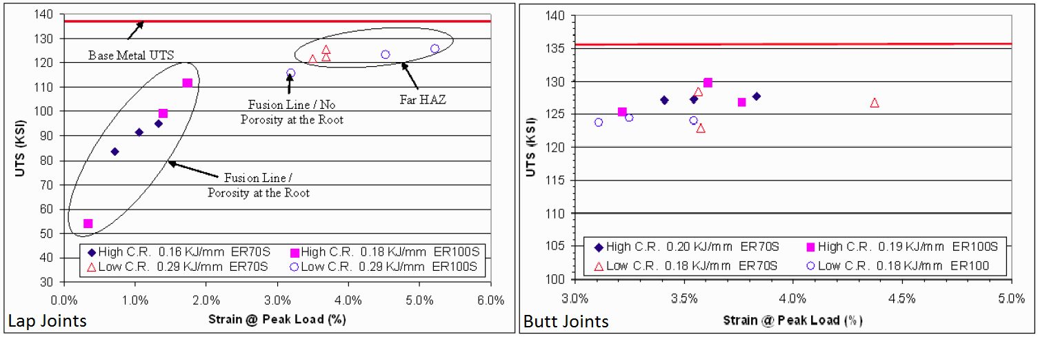
Figure 11: Dynamic tensile test results of TRIP 780 lap joints and butt joints.E-1
The dynamic tensile test results of the DP 780 butt joints are shown in Figure 12. All failed in the softened region of the far HAZ. UTS ranged from 841 to 910 MPa (122 to 132 ksi), and strain at peak load ranged from 2.25% to less than 4.0%. It should be noted that similar UTS were obtained for the DP 780 and TRIP 780 butt joints. On average, TRIP 780 butt joints had slightly higher strain at peak load. Neither filler metal strength nor CR condition appears to have a distinguishable effect on the dynamic tensile properties.
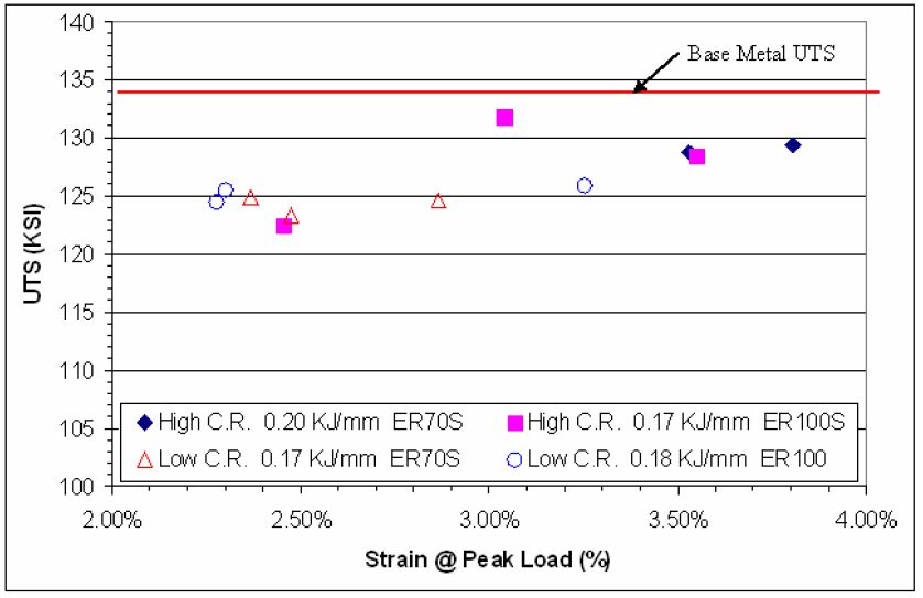
Figure 12: Dynamic tensile test results of DP 780 butt joints.E-1
Back To Top