Kate Hickey, Author at AHSS Guidelines

Twinning Induced Plasticity

TWinning Induced Plasticity (TWIP) steels have the highest strength-ductility combination of any steel used in automotive applications, with tensile strength typically exceeding 1000 MPa and elongation typically greater than 50%.

TWIP steels are alloyed with 12% to 30% manganese that causes the steel to be fully austenitic even at room temperature. Other common alloying additions include up to 3% silicon, up to 3% aluminum, and up to 1% carbon. Secondary alloying additions include chromium, copper, nitrogen, niobium, titanium, and/or vanadium.^D-29 The high alloying levels and substantially greater levels of strength and ductility place these into the 2nd Generation of Advanced High Strength Steels. Furthermore, due to the density of the major alloying additions relative to iron, TWIP steels have a density which is about 5% lower than most other steels.

Calling this type of steel TWIP originates from the characteristic deformation mode known as twinning. Deformation twins produced during sheet forming leads to microstructural refinement and high values of the instantaneous hardening rate (n-value). The resultant twin boundaries act like grain boundaries and strengthen the steel. On either side of a twin boundary, atoms are located in mirror image positions as indicated in the schematic microstructure shown in Figure 1. Figure 2 highlights the microstructure of TWIP steel after annealing and after deformation.

Figure 1: Schematic of TWIP steel microstructure.

Figure 2: TWIP steel in the annealed condition (left) and after deformation (right) showing deformation twins. The number of deformation twins increases with increasing strain.^K-42

EDDS or Interstitial-Free or Ultra-Low Carbon steels are different descriptions for the most formable lower-strength steel. Possible test results for this grade are 150 MPa yield strength, 300 MPa tensile strength, 22% to 25% uniform elongation, and 45% to 50% total elongation. In contrast, test results on TWIP steels may show 500 MPa yield strength, 1000 MPa tensile strength, 55% uniform elongation, and 60% total elongation.

The stress-strain curves for these two grades are compared in Figure 3. The TWIP curves show the manifestation of Dynamic Strain Aging (DSA), also known as the PLC effect, with more details to follow.

Figure 3: Uniaxial tensile stress-strain curves for an interstitial-free (IF) extra-deep-drawing steel and an austenitic Fe-18%Mn-0.6%C-1.5%Al TWIP steel. Curves are presented both terms of engineering (s,e) and true (σ,ε) stresses and strains, respectively.^D-30

Figure 4 compares the results of bulge testing ferritic interstitial-free (IF) steel and austenitic Fe-18%Mn-0.6%C-1.5%Al TWIP steel. The TWIP steel is still undamaged at a dome height that is 31% larger than the IF steel dome height at failure.^D-30

Figure 4: Comparison of dome testing between EDDS and TWIP.^D-30

Excellent stretch formability is associated with high n-values. Shown in Figure 5 is a plot showing how the instantaneous n-value changes with applied strain. N-value increases to a value of 0.45 at an approximate true (logarithmic) strain of 0.2 and then remains relatively constant until an approximate true strain of 0.3 before increasing again. The high and uniform n-value delays necking and minimizes strain peaks. Twins continue to form at higher strains, leading to finer microstructural features and continued increases in n-value at higher strains.

Figure 5: Instantaneous n-value changes with applied strain. TWIP steels have high and uniform n-value leading to excellent stretch formability.^C-30

A microstructural deformation phenomenon known as the Portevin-LeChatelier (PLC) effect occurs when deforming some TWIP steels to higher strain levels. The PLC effect is known by several other names as well, including jerky flow, discontinuous yielding, and dynamic strain aging (DSA).

The severity varies with alloy, strain rate, and deformation temperature. Figure 6 shows how DSA affects the appearance of the stress strain curve of two TWIP alloys.^D-29 The primary difference in the alloy design is the curves on the right are for steel containing 1.5% aluminum, with the curves on the left for a steel without aluminum. The addition of aluminum delays the serrated flow until higher levels of strain. Note that both alloys have negative strain rate sensitivity.

Figure 6: Influence of aluminum additions on serrated flow in Fe-18%Mn-0.6%C TWIP (Al-free on the left) and Fe-18%Mn-0.6%C-1.5% Al TWIP (Al-added on the right).^D-29

The primary macroscopic manifestations of the Portevin-LeChatelier (PLC) effect are^D-29:

negative strain rate sensitivity.
stress-strain curve showing serrated or jerky flow, indicating non-uniform deformation. Strain localization takes place in propagating or static deformation bands.
the strain rate within a localized band is typically one order of magnitude larger, while that outside the band is one order of magnitude lower, than the applied strain rate.
limited post-uniform elongation, meaning uniform elongation is just below total elongation. Said another way, fracture occurs soon after necking initiation.

The PLC effect leads to relatively poor sheared edge expansion, as measured in a hole expansion test. Figure 7 on the left highlights the crack initiation site in a sample of highly formable EDDS-IF steel, showing the classic necking appearance with extensive thinning prior to fracture. In contrast, note the absence of necking in the TWIP steel shown in the right image in Figure 7.^D-29

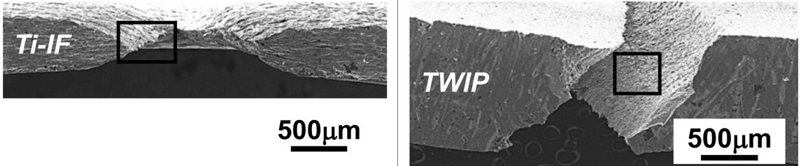
Figure 7: Sheared edge ductility comparison between IF (left) and TWIP (right) steel. TWIP steels lack the sheared edge expansion capability of IF steels.^D-29

The stress-strain curves of several TWIP grades are compared in Figure 8.

Figure 8: Engineering stress-strain curve for several TWIP Grades.P-30

Figure 8: Engineering stress-strain curve for several TWIP Grades.^P-18

Complex-shaped parts requiring energy absorption capability are among the candidates for TWIP steel application, Figure 9.

Figure 9: Potential TWIP Steel Applications.^N-24

Early automotive applications included the bumper beam of the 2011 Fiat Nuova Panda (Figure 10), resulting in a 28% weight savings and 22% cost savings^N-24 over the prior model which used a combination of PHS and DP steels.^D-31

Figure 10: Transitioning to a TWIP Bumper Beam Resulted in Weight and Cost Savings in the 2011 Fiat Nuova Panda. ^N-24^, ^D-31

In the 2014 Jeep Renegade BU/520, a welded blank combination of 1.3 mm and 1.8 mm TWIP 450/950 (Figure 11) replaced a two-piece aluminum component, aiding front end stability while reducing weight in a vehicle marketed for off-road applications.^D-31

Figure 11: A TWIP welded blank improved performance and lowered weight in the 2014 Jeep Renegade BU/520.^D-31

Also in 2014, the Renault EOLAB concept car where the A-Pillar Lower and the Sill Side Outer were stamped from TWIP 980 steel.^R-21By 2014, GM Daewoo used TWIP grades for A-Pillar Lowers and Front Side Members, and Hyundai used TWIP steel in 16 underbody parts. Ssangyong and Renault Samsung Motors used TWIP for Rear Side Members.^I-20

Other applications include shock absorber housings, floor cross-members, wheel disks and rims, wheelhouses, and door impact beams.

A consortium called TWIP4EU with members from steel producers, steel users, research centers, and simulation companies had the goal of developing a simulation framework to accurately model the complex deformation and forming behavior of TWIP steels. The targeted part prototype component was a backrest side member of a front seat, Figure 12. Results were published in 2015.^H-58

Figure 12: TWIP4EU Prototype Component formed from TWIP Steel.^H-58

In addition to a complex thermomechanical mill processing requirements and high alloying costs, producing TWIP grades is more complex than conventional grades. Contributing to the challenges of TWIP production is that steelmaking practices need to be adjusted to account for the types and amounts of alloying. For example, the typical ferromanganese grade used in the production of other grades has phosphorus levels detrimental to TWIP properties. In addition, high levels of manganese and aluminum may lead to forming MnO and Al₂O₃ oxides on the surface after annealing, which could influence zinc coating adhesion in a hot dip galvanizing line.^D-29

Bending

Forming Modes

top-of-page

Rotary Bending

The usual mode of bending is curvature around a straight-line radius (Figure 1). Through the thickness is a gradient of strains from maximum outer fiber tension (the outermost surface) through a neutral axis to inner fiber compression (the surface closest to the punch or bend axis). No strain occurs along the bend axis in the direction parallel to the bend axis, and therefore is in plane strain. The discussion below considers only bulk deformation, and excludes the implications of any edge effects. Bend testing procedures are linked here.

Figure 1: Typical bend where the outer surface is in tension, and the inner surface is in compression. A neutral axis lies in between.^S-23

When sheet metal flows through draw beads or over the die radius into the punch opening, it is bent, straightened, and in the case of draw beads re-bent in the opposite direction. The net strain after this process may be relatively small. However, each of the sequential bending and unbending steps strain hardens the sheet metal, which reduces the ability for further deformation of the metal in subsequent operations.

Deformation at the outer surface during three-point bending depends on the stretchability capacity of the metal. The failure strain in the bend is related to the total elongation of conventional steel, but AHSS grades with multiphase microstructures such as DP and TRIP experience shear fracture that severely reduces the bendability before failure occurs. A higher total elongation helps sustain a larger outer fiber stretch of the bend before surface fracture, thereby permitting a smaller bend radius. Since total elongation decreases with increasing strength for a given sheet thickness, the minimum design bend radius must be increased (Figure 2).

Figure 2: Larger bend radius is needed as the total elongation decreases.^S-23

The ratio of punch radius to sheet thickness, or the r/t ratio, allows for calculation of the amount of elongation on the outermost surface. This value can be compared against the total elongation of the metal as determined in a tensile test, or against the minimum elongation value allowed in the specification. If the part geometry will not allow for sufficient elongation for the selected metal grade, then either the part, process, or steel grade must change. [Note that this is not a perfect assessment, since elongation in a tensile test is measured relative to a 50 or 80 mm gauge length, which is likely different than the dimensions of the bent section.]

For design and springback control, usually a smaller r/t ratio is desirable. However, this may not be suitable in terms of formability. Increased material strength usually is associated with a reduction in total elongation, which in turn means a successful bend requires a larger r/t ratio.

For equal strengths, most AHSS grades have higher total elongations than conventional HSLA steels. However, several AHSS grades have limited local formability based on their microstructure, and may be at risk for cracking during edge expansion.

Cracking in production stamping conditions at stress levels below what is predicted with Forming Limit Diagrams may be attributed to these local formability failures. As an illustration, physical bend tests and simulations were performed for both HSLA and DP780 steels.^S-11 The HSLA global formability failure aligned with simulation predictions (Figure 3), and was accompanied by a visible neck (Figure 4). In contrast, the DP780 showed no visible neck at the failure site (Figure 5) and no correlation between the simulation and actual test results (Figure 6).

Like hole expansion, bending limits in AHSS products are further lowered by shear fracture associated with the interfaces between the ductile ferrite and the hard martensite phase in the microstructure. This reduction becomes more severe as the strength increases, since increasing strength is achieved by increasing the volume of the hard martensite phase. More about shear fracture is found here.

Figure 3: Forming simulation of HSLA with strong correlation to actual testing.^S-11

Figure 4: Close-up of visible necking before tensile failure in HSLA.^S-11

Figure 5: Comparison of forming simulation with actual testing of the DP780. Note lack of correlation.^S-11

Figure 6: Close-up of local formability failure on DP780 with no visible necking before failure.^S-11

Rotary Bending

One way to address springback involves the use of rotary benders. Rotary benders transfer the vertical movement of a press stroke into a precise, rotary forming motion. A rocker or rotating die can simultaneously hold, bend, and overbend the sheet past 90° to counter material springback (Figure 7).

Figure 7: The rotation of the rocker bends the sheet metal around the anvil with less pressure than needed for wipe tools^D-8

Use rotary bending tooling where possible instead of flange wipe dies. Rotary bending allows for easy adjustment of the bending angle to correct for changes in springback due to variations in steel properties, die set, lubrication, and other process parameters. In addition, the tensile loading generated by the wiping shoe is absent.

There are four sequential steps to the process:
1) Downward pressure from the rocker clamps the part with the bending lobes before bending starts
2) Induced rotation of the rocker bends material around the anvil
3) The rocker bends the sheet metal past final angle to compensate for springback
4) The rocker releases the sheet metal to allow springback to desired angle

Using rotary benders to roll darts into the part during bending provides another way to reduce springback and stiffen the part (Figure 8).

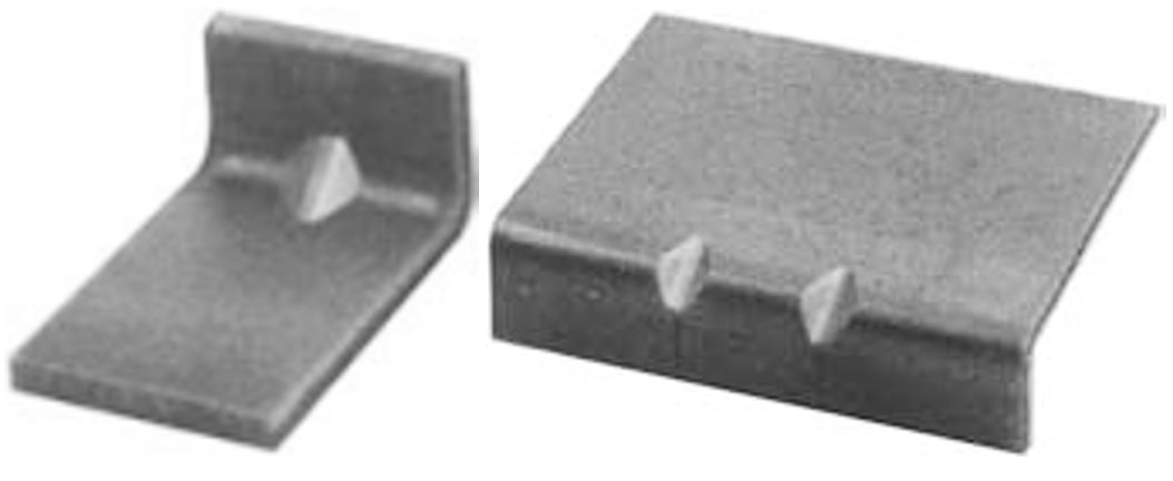
Figure 2: Stiffening darts can be created as part of the rotary bending operation.R-7

Figure 8: Stiffening darts can be created as part of the rotary bending operation.^R-7

Back to the Top

Rotary Bending

Shear Affected Zone

Cutting, Cutting-Blanking-Shearing-Trimming

A cut edge has four distinct zones with different characteristics:

Rollover – The plastically deformed zone bent as the cutting tools contact the edge of the sheet surface.
Burnish – The zone where the cutting tools penetrate into the sheet metal, prior to any fracturing. The sheet metal stresses are such that the surface compresses into the cutting tool, which gives it a flat, smooth, and shiny appearance. The shear zone is another name for this region.
Fracture – The zone where the cutting steels fracture the sheet metal, leading to separation from the remainder of the sheet. The surface of this region is rougher than the burnish zone, and is at an angle from the cutting direction.
Burr – The metal elongated and pushed out on the trailing edge of the cut.

The cutting process also deforms the metal near the shear face, creating what is known as the shear affected zone (SAZ). The degree and influence of this deformation is a function of the cutting process (shearing, water jet, laser, and so on) as well as the steel microstructure and strength. Many studies conclude plastic deformation within the SAZ is a key contributor to sheared edge stretching failures.

The Shear Affected Zone is the area of work-hardened steel and microstructural damage behind the sheared edge. The deformation pattern in the SAZ includes a large shear-induced rotation of the grains that increases with proximity to the sheared edge. An etched cross-section such as that shown in Figure 1 highlights the grain rotation and gives a visual indication of the size of the zone.

Figure 1: Shear Face Components and Shear Affected Zone.^K-1

Work hardening in the SAZ leads to a way to quantify the depth of the SAZ: by creating a hardness profile with readings starting at the edge and progressing deeper into the metal. The end of the SAZ occurs when the hardness readings level off to the bulk hardness.

Figure 2 compares the edge and hardness readings for CP800 and DP780, showing the depth of the SAZ for DP780 is about 41% of the initial sheet thickness of 1.56 mm, and the depth of the CP800 SAZ is 20% of the initial 2.90 mm sheet thickness.^P-12

Figure 2: A) Sheared edge and SAZ of CP800; B) Sheared edge and SAZ of DP780; C) CP800 microstructure away from edge; D) DP780 microstructure away from sheared edge; E) hardness profile for the two sheared edges in the rolling direction.^P-12

Plastic deformation from cutting and subsequent edge expansion forms micro-voids and creates other microstructural damage. The voids grow and combine with neighboring voids to create micro-cracks, which in turn combine with other micro-cracks resulting in the cracks that cause fractures in stampings.

Void nucleation in DP steels occurs through two mechanisms: decohesion of the ferrite-martensite interface or fracture of martensite islands.^P-12^{, A-27,} ^A-28 Figure 3 shows an example of both.

Figure 3: Aligned voids along loading direction. White solid square shows interface damage between martensite and ferrite. White dashed circles show voids formed by cracking of martensite.^A-28

The study in Citation P-12 compared CP800 and DP780. The CP800 microstructure contains ferrite, bainite, and martensite. The DP780 microstructure has more martensite, with a larger strength differential between the phases, which combines to result in a lower nucleation strain and accelerated void nucleation compared with CP800. The DP grade has a larger SAZ, further promoting nucleation, growth, and coalescence of voids. This results in failure at a lower strain and leads to the lower edge stretchability of the DP780 compared to the CP800 alloy.^P-12 The ductility of bainite restrains void initiation at high strains, which may play a role in improved sheared edge performance.^{S-24, S-25}

Fracture initiation energy, a measure of fracture toughness correlates with hole expansion and stretch-ﬂangeability as shown in Figure 4.^Y-5

$Figure 4: Correlation between fracture initiation energy and hole expansion ratio of various metals. Steels A – D are AHSS grades with Tensile strength ranging from 725 – 1000 MPa.Y-5$

Figure 4: Correlation between fracture initiation energy and hole expansion ratio of various metals. Steels A – D are AHSS grades with Tensile strength ranging from 725 – 1000 MPa.^Y-5

In addition to microstructural damage and fracture mechanics, simulation models improve in accuracy when the incorporating the effect of the temperature increase in the localized deformation zone. Simulation of the blanking of AISI 1050 shows a temperature at the cut edge of 440 °C. The edge temperature may be even higher in AHSS grades due to their higher strength.^A-29

Figure 5: 1.27mm AISI 1050 steel blanked with 15% clearance. The simulation shows temperature, with the cut face getting as hot as 440 °C.^A-29

When factoring in the considerations described here, simulation accuracy of hole expansion and sheared edge stretching improves significantly. Citations L-13 and L-14 provide additional background information about the Shear Affected Zone.

Non-Linear Strain Paths (Stress-Based FLCs)

FLC and FLD

Conventional Forming Limit Curves (FLCs) gained widespread industrial use since being introduced by Dr. Stuart Keeler in the 1960’s. Applications from feasibility analysis to stamping plant troubleshooting use these principles. The strain hardening exponent (n-value) and thickness are inputs into a shortcut to create the curve placement and shape, but this is applicable to only mild steels, conventional High-Strength Steels, and some Advanced High-Strength Steels. Furthermore, this shortcut is an approximation, coming from a best-fit curve generated from data points gathered over multiple grades.

A typical method used in creating most FLCs includes deforming samples of different widths with a 100 mm (4 inch) diameter hemispherical punch – known as the Nakajima method. An alternate approach uses a flat-bottom cylindrical punch, known as the Marciniak method (Figure 1). Independent of the punch shape used, generating FLCs involves measuring the strains resulting from deforming a blank to a formed shape. The conventional FLC plots major strain on the vertical axis against minor strain on the horizontal axis. This FLC applies only to in-plane stretching in linear strain paths, and assumes that there are no through-thickness stress or strain differences. Assessing bendability or cut edge ductility is not possible with this approach.

Figure 1: Punch Shape Used to Create Forming Limit Curves Result in Through-Thickness Strain Differences Which Influence the Shape and Placement of The FLC [Reference 1]

Figure 1: Punch Shape Used to Create FLCs Result in Through-Thickness Strain Differences Which Influence the Shape and Placement of The FLC ^S-37

Figure 2 compares the FLCs generated by deforming DP980 with the three punch shapes highlighted in Figure 1. Note the higher strains associated with the 50 mm diameter hemispherical punch compared with the strains generated from the 100 mm diameter hemispherical punch. This punch curvature difference impacts the magnitude of the strains that develop through the thickness of the sheet. On samples deformed with a hemispherical punch, the selected strain measurement technique (circle/square grid analysis or Digital Image Correlation, for example) directly measures strains on the outer top surface only, with the middle and inner surface having progressively lower strains as a function of the R/T ratio. A punch or feature with small R/T leads to high strains on the outermost surface. Strains exceeding the FLC on only this outer surface will not lead to necks on the formed panel. Exceeding the FLC through the entire thickness – from the inner surface to the outer surface – must occur for the sample to show a neck.^T-17

Figure 2: FLCs of the same batch of DP980 Showing Dependence on Punch Shape and Curvature [References 1 and 3]

Figure 2: FLCs of the same batch of DP980 Showing Dependence on Punch Shape and Curvature.^S-37, ^M-15

In addition to the through-thickness strain differences from the punch curvature, the metal flow differences resulting from the punch shapes leads to directional changes in the strain path taken by the deforming metal. A channel drawn part with a hat-shaped cross section in which there are no features like embossments is likely to have a linear strain path. Forming every other engineered stamped part geometry involves some degree of a non-linear strain path (NLSP).

The importance of strain path and deformation history comes from the changes in the forming limit that occur once metal deformation starts. The black curve in Figure 3 shows the FLC for an alloy generated in a conventional manner with as-received metal, assuming a linear strain path. The red curve results from testing the same metal that initially stretched to an equal-biaxial plastic pre-strain of 0.07. In this strain path, substantially less deformation can occur before reaching the forming limit. However, the strain path changes if the local part contour is different, and that strain path results in a different amount of subsequent deformation prior to necking. The magnitude and direction of the shift changes based on the strain and the orientation relative to the rolling direction. Citation S-38 highlights these curves and presents more examples of the effects of different strain paths. The important conclusion is that the amount of deformation that a metal is capable of withstanding prior to necking changes throughout the forming process and depends on the local part shape (among other variables), and cannot be discerned by using only the conventional strain based FLC.

Figure 3: Experimental FLCs for a linear strain path (in black) and for a bilinear strain path after 0.07 strain in equal biaxial tension in strain space (in red) ^S-38

Figure 4 shows the strain paths associated with the FLCs presented in Figure 2, with along with a magnified portion of one of the curves. This non-linearity is a characteristic of samples formed with a dome, associated with the sample wrapping around the punch during the initial contact and experiencing a combination of biaxial bending and stretching. Citation M-15 presents a method to correct for strain path effects.

Figure 4: Strain Path for FLCs shown in Figure 2. A) 100 mm diameter flat punch; B) 100 mm diameter hemispherical punch; C) 50 mm diameter hemispherical punch; and D) Magnified portion of one curve from Figure 4B showing the non-linearity of the strain path.^S-37, ^M-15

Accounting for tool contact pressure is critical as well, since pressure through the sheet thickness suppresses the onset of necking. Applying this compensated FLC in simulation or in hands-on analysis parts analysis requires modification for the unique characteristics of each part, with appropriate adjustments for local curvature, contact pressure and deformation history. Citations S-37 and M-15 detail methods to compensate for the effects of strain path, curvature, and tool pressure. Figure 5 shows that after incorporating these corrections, the curves condense to one shape independent of the variables used.

Figure 5: As-generated FLCs compared with FLCs after strain path, curvature, and tool contact pressure corrections [References 1 and 3]

Figure 5: As-generated FLCs compared with FLCs after strain path, curvature, and tool contact pressure corrections.^S-37, ^M-15

In summary, FLCs generated from relatively similar simple tools are sensitive to small differences in R/T ratio, incorporation of tool contact pressure, and deviations from a linear strain path. By comparison, engineered stampings require substantially more complex tool shapes with differing degrees of curvature, tool contact pressure, and strain paths all within one part. These complex part shapes contribute to an even wider variation in the yield surface and hardening mechanisms important for simulation, and impacts predictions of formability, springback, and stress analysis.

A common requirement during tooling buyoff – where all strains need to be below the FLC by at least a certain amount called the safety margin – magnifies these challenges. AHSS grades already have low FLCs relative to their lower strength counterparts, so it is critical that the chosen FLC does not further reduce efficient application of these grades. Minimizing sensitivity to the changes in strain path occurring across a complex part requires using a different approach – a FLC with the axes in stress-space rather than the conventional strain-space.

This discussion has centered on conventional strain-based FLCs, which incorporate an assumption of a linear strain path as a flat sheet deforms to the final shape. Stress-based Forming Limit Curves (sFLC or FLSC) are insensitive to deformation history and can be adjusted to reflect the differences in local tool geometry or contact pressure across the stamping. Forming analysis software readily converts conventional FLCs into stress-based units. Figure 6 converts the two strain paths presented in Figure 3 into stress-space, and shows the two experimental stress FLCs generated with different strain paths are independent of the loading history and essentially overlap. Citations S-38, S-39, S-40 and S-41 contain information about stress-based FLCs, as well as their generation and usage.

Figure 6: After converting the conventional FLCs in Figure 3 to stress-space, the experimental stress-based FLCs show no significant differences.^S-38

Citation H-20 presents a related method to transition from strain-based to stress-based Forming Limit Curves. The proposed stress-based failure criterion postulates that localized necking occurs when a critical normal stress condition is met. This approach adequately describe the experimental strain-based forming limit data in most evaluated materials, failing only with a 3rd Generation AHSS alloy containing a high percentage of retained austenite. For this grade, the authors speculate that a material model more advanced than the one employed in this study will improve correlation.

Accurate simulation requires accurate and complete inputs, including the full range of metal properties, with correct material flow and hardening models, and an understanding of the conditions that will produce failure. Any shortcuts taken increases the likelihood that simulation will not fully match reality for all materials, part shapes, and production processes. A conventional strain-based FLC assumes no effect of part geometry, tool contact pressure, and deformation history – all of which occur on engineered stampings to differing degrees. Analysts should incorporate stress-based FLCs into their simulation with appropriate adjustments to address local geometry and contact pressure to ensure an accurate representation of the metal’s forming characteristics.

For use in the die shop or stamping plant, a growing number of optical systems have built-in features to map strain measurements on to an sFLC. Use caution when employing this approach since these systems measure only the final net strain, and not the strain history as the panel deforms. Proper application involves capturing metal flow from individual breakdown panels and adjusting the FLC accordingly as the panel gets closer to the home position.

Special thanks to Dr. Thomas Stoughton, Technical Fellow, General Motors Research & Development, for assistance in preparing this information.

Drawing

Forming Modes

Drawing is the sheet metal forming process where the punch that creates the part shape forces the sheet metal to pull in from the flange area. In contrast with stretch-drawing or stretch forming, little metal thinning occurs in pure drawing. There is not a generally accepted definition for the term “deep drawing,” although some references describe it as when the depth of draw is greater than the diameter.

Drawability, or the ability for a sheet metal to be drawn into a cup, is assessed by the cup drawing test to measure the Limiting Draw Ratio, or LDR. Here, a cylindrical punch contacts and then pushes a circular blank into the die (Figure 1). The ratio of the largest blank diameter successfully drawn into a cup to the punch diameter used for drawing is the LDR.

Figure 1: In the cup drawing test, a punch deforms a circular blank into a cylindrical cup. The largest ratio of blank diameter to punch diameter successfully drawn into a cup is the Limiting Draw Ratio (LDR).

In the LDR test, metal in the circular blank flows over the die radius and into the cup wall. The metal movement from the flat blank to the vertical sidewalls is the only metal movement which happens, since there is no metal flow within the flat bottom region.

As shown in Figure 2, the flange of the circular blank undergoes radial tension and a circumferential compression as the flange moves in a radial direction towards the circular die radius in response to a pull generated by a flat bottom punch. Blank holder pressure is set to prevent buckles in the blank.

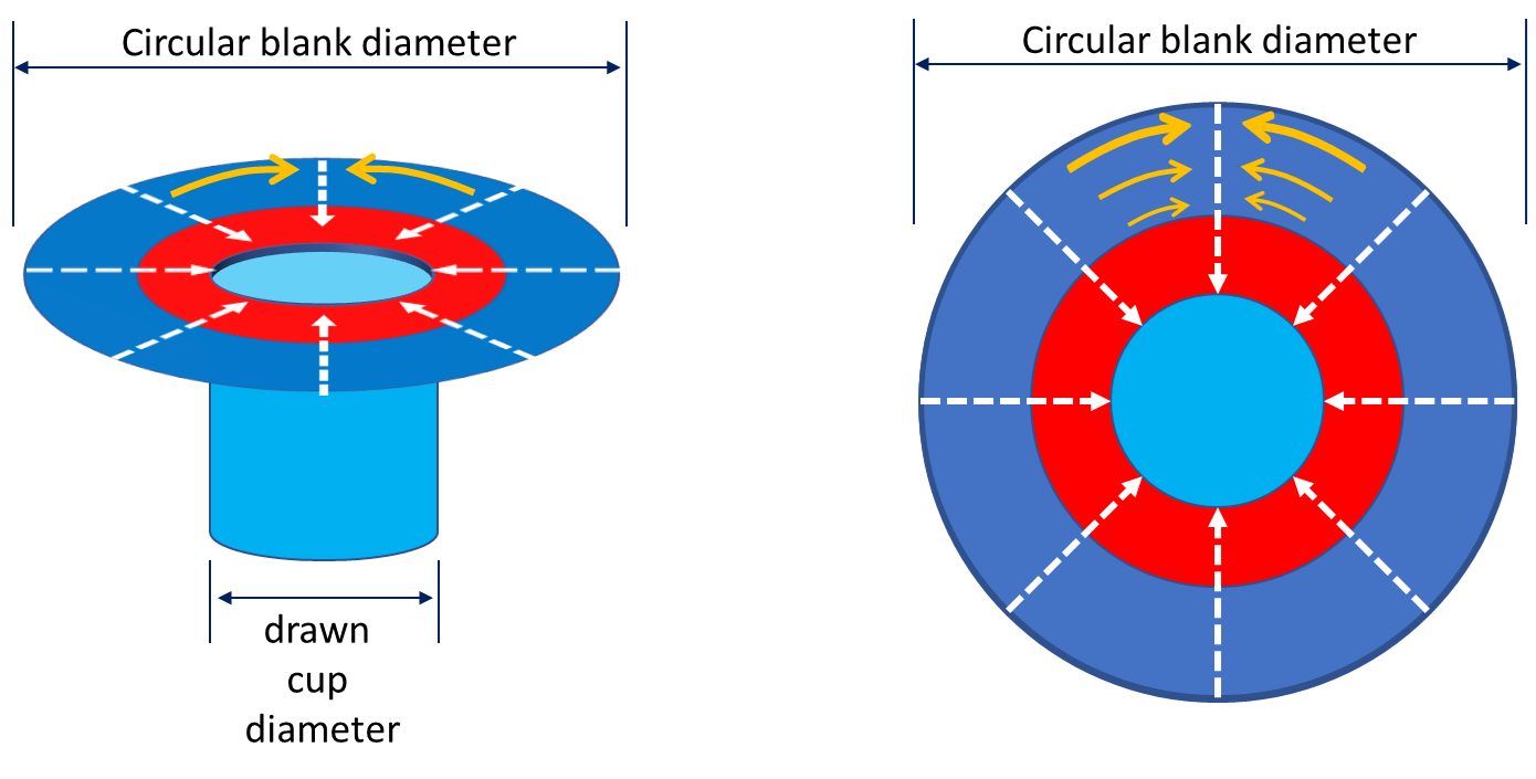
Figure 2: Tension and compression in a drawn cup. Dashed white arrows indicate the radial tension created during cup forming; orange arrows indicate flange compression as a greater amount of metal feeds into progressively smaller regions.

The steel property that improves cup drawing or radial drawing is the normal anisotropy or r_m value. Values greater than 1 increase in the Limiting Draw Ratio. In contrast, the LDR is insensitive to the strength of the steel and the n-value. High-strength steels with UTS greater than 450 MPa and hot-rolled steels have r_m values approximating one and LDR values between 2.0 – 2.2. Therefore, DP and HSLA steels have similar LDR values. However, TRIP steels have a slightly improved LDR deep drawability.^T-2 Since the transformation of retained austenite to martensite is influenced by the deformation mode (Figure 3), the amount of transformed austenite to martensite generated by shrink flanging in the flange area is less than the plane strain deformation in the cup wall. This difference in transformation from retained austenite to martensite makes the wall area stronger than the flange area, thereby increasing the LDR. The benefit of the increased LDR is seen in Figure 4 which shows cups formed from different grades having the same tensile strength.

Figure 3: The cup wall in plane strain strengthens more than the shrink flange due to increased amounts of transformed martensite in TRIP steels.^T-2

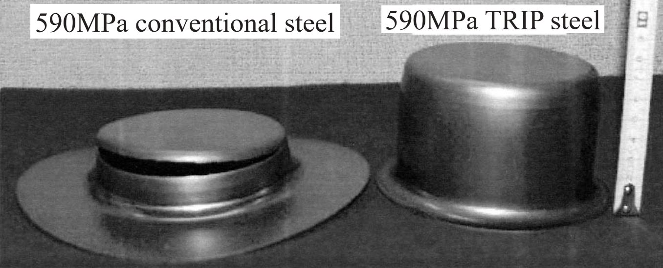
Figure 4: Cups formed from 590MPa tensile strength steels, highlighting greater draw depths possible with TRIP steels.^T-2

In a study of different grades^C-9, laboratory cup drawing experiments show an approximate LDR of 2.0 – 2.2 for the DP steels tested (Figure 5). Note that a doubling of the yield strength has no effect on the LDR. An increased r_m value of mild steel created a small increase in LDR over DP steel. The LDR of the MS (martensitic) steel evaluated may have been impacted by the reduced bendability going over the die radius. Figure 6 shows the cup draw depths possible for the grades reported in Figure 5.^S-26

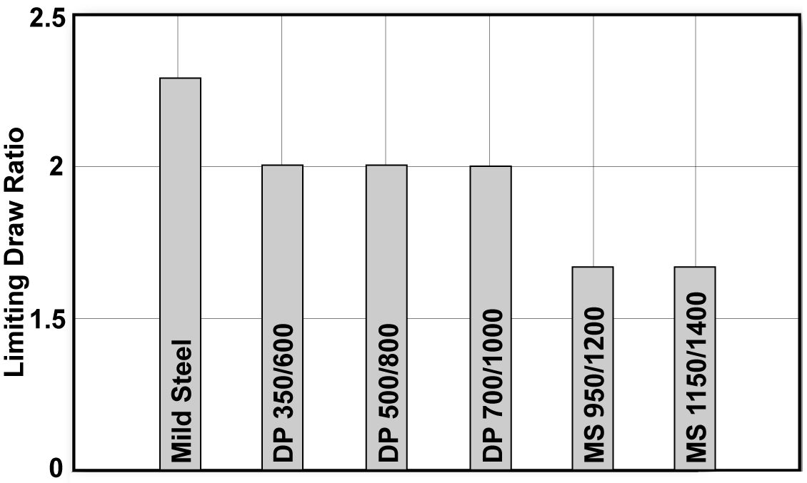
Figure 5: LDR tests for Mild, DP, and MS steels.^C-9

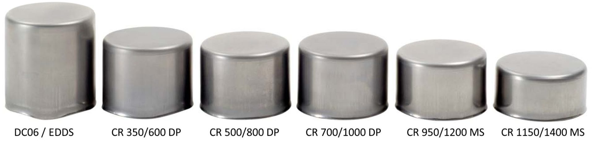
Figure 6: Cups used in the testing reported in Figure 5.^S-26

Even though r-value is the only steel property influencing the formability of drawn flat-bottom cups through its relationship with LDR, not all cups have flat bottoms. Some have hemispherical or other configurations for bottoms. Adding a dome-like shape to the cup results in a more complex forming operation which is now sensitive to material properties like n-value and microstructures.

Corners of box-shaped stampings and the ends of closed channels contain design features similar to drawn cups, providing insight on an analytical approach.

The four corners of a box-shaped drawn panel should each be analyzed as one-quarter of a cup. Buckles forming in the binder area indicate compressive flow. The corners of the blank will form the same as a deep drawn cup.
The side walls are formed by metal flowing from the binder across the die radius. The term for this metal flow is bend-and-straighten.

In summary, higher LDR values are achievable in steels with greater values of the normal anisotropy ratio, r_m. The absolute value of the LDR, however, also depends on the lubrication, blank holder load, die radius and other system inputs. Figure 7 compares a higher viscosity lubricant on the left with a lower viscosity lubricant on the right.^S-26 Die radii need to be balanced: large radii promotes metal flow and may lead to wrinkles, while small radii restricts metal flow and may lead to splits.

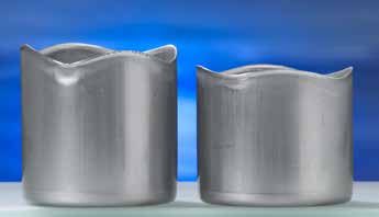
Figure 7: The influence of lubricant viscosity on drawing. The cup formed with the higher viscosity lubricant is on the left.^S-26

« Older Entries

Next Entries »