![Elastic Modulus]()
Mechanical Properties
Elastic Modulus (Young’s Modulus)
When a punch initially contacts a sheet metal blank, the forces produced move the sheet metal atoms away from their neutral state and the blank begins to deform. At the atomic level, these forces are called elastic stresses and the deformation is called elastic strain. Forces within the atomic cell are extremely strong: high values of elastic stress results in only small magnitudes of elastic strain. If the force is removed while causing only elastic strain, atoms return to their original lattice position, with no permanent or plastic deformation. The stresses and strains are now at zero.
A stress-strain curve plots stress on the vertical axis, while strain is shown on the horizontal axis (see Figure 2 in Mechanical Properties). At the beginning of this curve, all metals have a characteristic linear relationship between stress and strain. In this linear region, the slope of elastic stress plotted against elastic strain is called the Elastic Modulus or Young’s Modulus or the Modulus of Elasticity, and is typically abbreviated as E. There is a proportional relationship between stress and strain in this section of the stress-strain curve; the strain becomes non-proportional with the onset of plastic (permanent) deformation (see Figure 1).

Figure 1: The Elastic Modulus is the Slope of the Stress-Strain Curve before plastic deformation begins.
The slope of the modulus line depends on the atomic structure of the metal. Most steels have an atomic unit cell of nine iron atoms – one on each corner of the cube and one in the center of the cube. This is described as a Body Centered Cubic (BCC) structure. The common value for the slope of steel is 210 GPa (30 million psi). In contrast, aluminum and many other non-ferrous metals have 14 atoms as part of the atomic unit cell – one on each corner of the cube and one on each face of the cube. This is referred to as a Face Centered Cubic (FCC) atomic structure. Many aluminum alloys have an elastic modulus of approximately 70 GPa (10 million psi).
Under full press load at bottom dead center, the deformed panel shape is the result of the combination of elastic stress and strain and plastic stress and strain. Removing the forming forces allows the elastic stress and strain to return to zero. The permanent deformation of the sheet metal blank is the formed part coming out of the press, with the release of the elastic stress and strain being the root cause of the detrimental shape phenomenon known as springback. Minimizing or eliminating springback is critical to achieve consistent stamping shape and dimensions.
Depending on panel and process design, some elastic stresses may not be eliminated when the draw panel is removed from the draw press. The elastic stress remaining in the stamping is called residual stress or trapped stress. Any additional change to the stamped panel condition (like trimming, hole punching, bracket welding, reshaping, or other plastic deformation) may change the amount and distribution of residual stresses and therefore potentially change the stamping shape and dimensions.
The amount of springback is inversely proportional to the modulus of elasticity. Therefore, for the same yield stress, steel with three times the modulus of aluminum will have one-third the amount of springback.
Elastic Modulus Variation and Degradation
Analysts often treat the Elastic Modulus as a constant. However, Elastic Modulus varies as a function of orientation relative to the rolling direction (Figure 2). Complicating matters is that this effect changes based on the selected metal grade.

Figure 2: Modulus of Elasticity as a Function of Orientation for Several Grades (Drawing Steel, DP 590, DP 980, DP 1180, and MS 1700) D-11
It is well known that the Bauschinger Effect leads to changes in the Elastic Modulus, and therefore impacts springback. Elastic Modulus determined in the loading portion of the stress-strain curve differs from that determined in the unloading portion. In addition, increasing prestrain lowers the Elastic Modulus, with significant implications for forming and springback simulation accuracy. In DP780, 11% strain resulted in a 28% decrease in the Elastic Modulus, as shown in Figure 3.K-7

Figure 3: Variation of the loading and unloading apparent modulus with strain for DP780K-7
Another study documented the modulus degradation for many steel grades, including mild steel, conventional high strength steels, and several AHSS products.W-10 Data in some of the grades is limited to small plastic strains, since valid data can be obtained from uniaxial tensile testing only through uniform elongation.
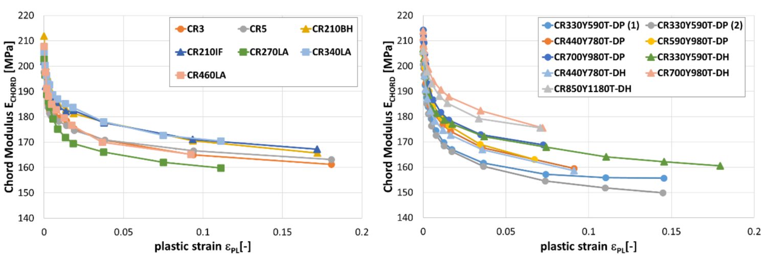
Reduction in chord modulus for mild steels and conventional high strength steels (left) and for DP and DH steels (right).W-10
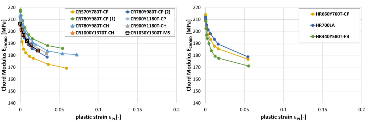
Reduction in chord modulus for CP, CH and MS steels (left) and for a selected of hot rolled steels (right).W-10
Blog, RSW Modelling and Performance
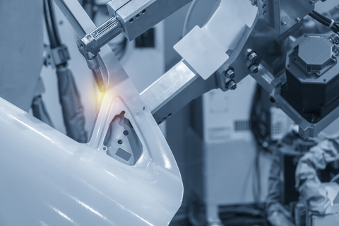
Modern car bodies today are made of increasing volumes of Advanced High-Strength Steels (AHSS), the superb performance of which facilitates lightweighting concepts (see Figure 1). To join the different parts of a car body and create the crash structure, the components are usually welded to achieve a reliable connection. The most prominent welding process in automotive production is resistance spot welding. It is known for its great robustness, and easily applicable in fully automated production lines.
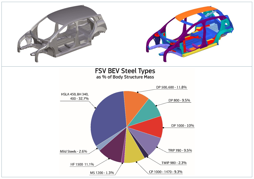
Figure 1: AHSS Content in Modern Car Body.W-7
There are, however, challenges to be met to guarantee a high-quality joint when the boundary conditions change, for example, when new material grades are introduced. Interaction of a liquefied zinc coating and a steel substrate can lead to small surface cracks during resistance spot welding of current AHSS, as shown in Figure 2. This so-called liquid metal embrittlement (LME) cracking is mainly governed by grain boundary penetration with zinc, and tensile stresses. The latter may be induced by various sources during the manufacturing process, especially under ‘rough’ industrial conditions. But currently, there is a lack of knowledge, regarding what is ‘rough’, and what conditions may still be tolerable.
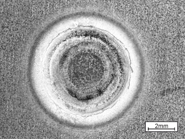
Figure 2: Top View of LME-Afflicted Spot Weld.
The material-specific amount of tensile stresses necessary for LME enforcement can be determined by the experimental procedure ‘welding under external load’. The idea of this method, which is commonly used for comparing cracking susceptibilities of different materials to each other, is to apply increasing levels of tensile stresses to a sample during the welding process and monitor the reaction. Figure 3 shows the corresponding experimental setup.

Figure 3: Welding under external load setup.L-51
However, the known externally applied stresses are not exclusively responsible for LME, but also the welding process itself, which puts both thermally and mechanically induced stresses/strains on the sample. Here, the conventional measuring techniques fail. A numerical reproduction of the experiment grants access to the temperature, stress and strain fields present during the procedure, providing insights on the formation of LME. The electro-thermomechanical simulation model is described in detail in Modelling RSW of AHSS. It is used to simulate the welding under external load procedure (see Figure 4).
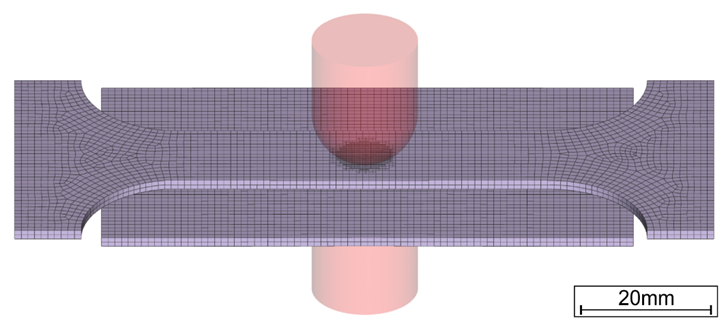
Figure 4: Simulation Model of Welding Under External Load.
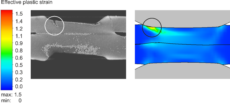
The videos that can be found in the link above show the corresponding temperature and plastic strain fields. As heat dissipates quickly through the water-cooled electrode, a temperature gradient towards the adjacent areas and a local temperature maximum on the surface forms. The plastic strains accumulate mainly at the electrode indentation area. The simulated strain field shows a local maximum of plastic deformation at the left edge of the electrode indentation, amplified by the externally applied stresses and the boundary conditions implied by the procedure. This area correlates with experimentally observed LME cracking sites and paths as shown in Figure 5.
The simulation shows that significant plastic strains are present during welding. When external stresses (in reality e.g. due to poor part fit-up or distorted parts) contribute to the already high load, LME cracking becomes more likely. The numerical simulation model facilitates the determination of material-specific safety limits regarding LME cracking. Parameter variations and their effects on the LME susceptibility can easily be investigated by use of the model, enabling the user to develop strict processing protocols to reduce the likelihood of LME. Finally, these experimental procedures can be adapted to other high-strength materials, to aid their application understanding and industrial set-up conditions.
Figure 5: LME Cracks in Cross Section View at Highly Strained Locations.
For more information on this topic, see the paper, co-authored by Fraunhofer and LWF Paderborn, documented in Citation F-23. You may also download the full report documenting the WorldAutoSteel LME project for which this work was conducted.
Blog, main-blog, RSW Modelling and Performance
Modelling resistance spot welding can help to understand the process and drive innovation by asking the right questions and giving new viewpoints outside of limited experimental trials. The models can calculate industrial-scale automotive assemblies and allow visualization of the highly dynamic interplay between mechanical forces, electrical currents and thermal flow during welding. Applications of such models allow efficient weldability tests necessary for new material-thickness combinations, thus well-suited for applications involving Advanced High -Strength Steels (AHSS).
Virtual resistance spot weld tests can narrow down the parameter space and reduce the amount of experiments, material consumed as well as personnel- and machine- time. They can also highlight necessary process modifications, for example the greater electrode force required by AHSS, or the impact of hold times and nugget geometry. Other applications are the evaluation of whole-part distortion to ensure good part-clearance and the investigation of stress, strain and temperature as they occur during welding. This more research-focused application is useful to study phenomena arising around the weld such as the formation of unwanted phases or cracks.
Modern Finite-Element resistance spot welding models account for electric heating, mechanical forces and heat flow into the surrounding part and the electrodes. The video shows the simulated temperature in a cross-section for two 1.5 mm DP1000 sheets:
First, the electrodes close and then heat starts to form due to the electric current flow and agglomerates over time. The dark-red area around the sheet-sheet interface represents the molten zone, where the nugget forms after cooling. While the simulated temperature field looks plausible at first glance, the question is how to make sure that the model calculates the physically correct results. To ensure that the simulation is reliable, the user needs to understand how it works and needs to validate the simulation results against experimental tests. In this text, we will discuss which inputs and tests are needed for a basic resistance spot welding model.
At the base of the simulation stands an electro-thermomechanical resistance spot welding model. Today, there are several Finite Element software producers offering pre-made models that facilitate the input and interpretation of the data. First tests in a new software should be conducted with as many known variables as possible, i.e., a commonly used material, a weld with a lot of experimental data available etc.
As first input, a reliable material data set is required for all involved sheets. The data set must include thermal conductivity and capacity, mechanical properties like Young’s modulus, tensile strength, plastic flow behavior and the thermal expansion coefficient, as well as the electrical conductivity. As the material properties change drastically with temperature, temperature dependent data is necessary at least until 800°C. For more commonly used steels, high quality data sets are usually available in the literature or in software databases. For special materials, values for a different material of the same class can be scaled to the respective strength levels. In any case, a few tests should be conducted to make sure that the given material matches the data set. The next Figure shows an exemplary material data set for a DP1000. Most of the values were measured for a DP600 and scaled, but the changes for the thermal and electrical properties within a material class are usually small.
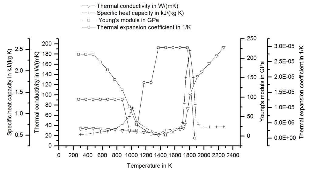
Figure 1: Material Data set for a DP1000.S-73
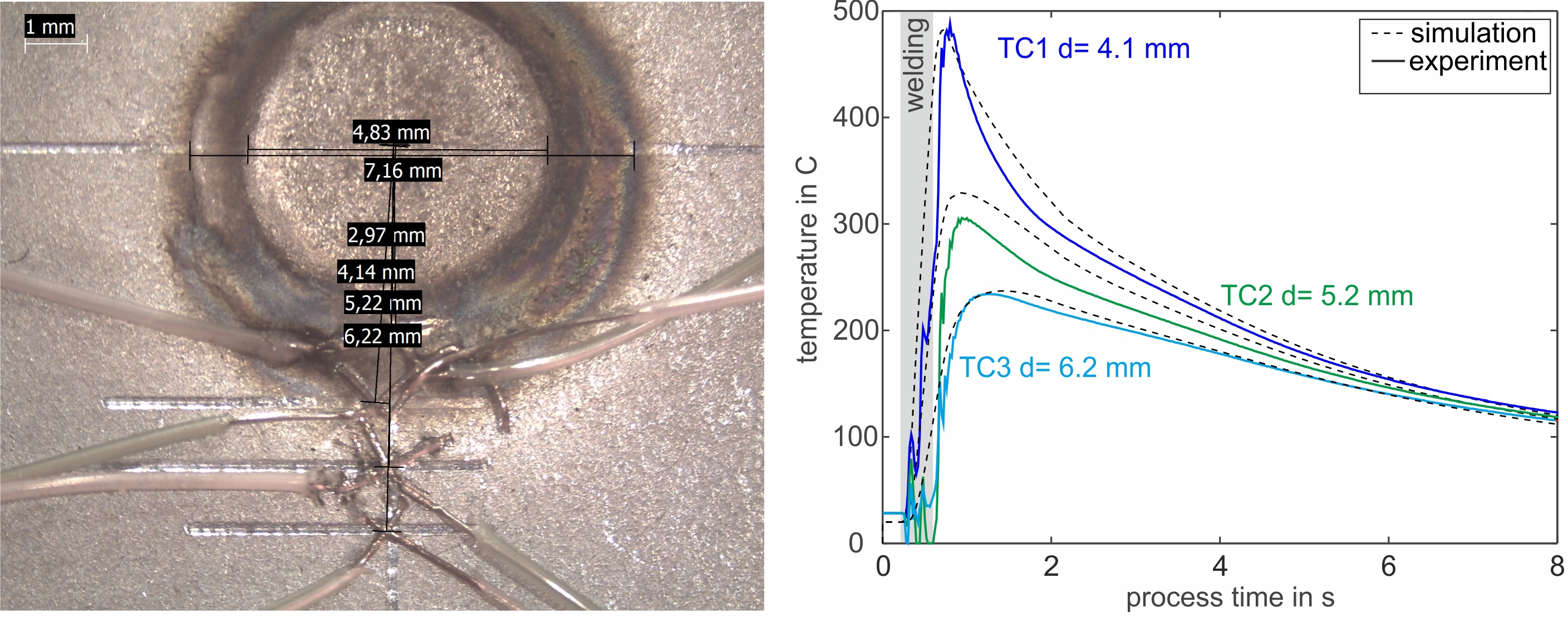
Next, meaningful boundary conditions must be chosen and validated against experiments. These include both the electrode cooling and the electrical contact resistance. To set up the thermal flow into the electrode, temperature measurements on the surface are common. In the following picture, a measurement with thermocouples during welding and the corresponding result is shown. By adjusting the thermal boundary in the model, the simulated temperatures are adjusted until a good match between simulation and experiment is visible. This calibration needs to be conducted only once when the model is established because the thermal boundary remains relatively constant for different materials and coatings.
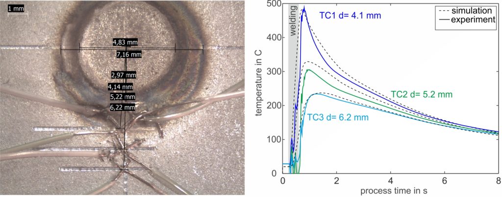
Figure 2: Temperature measurement with thermocouples during welding and the results. The simulated temperature development is compared to the experimental curve and can be adjusted via the boundary conditions.F-23
The second boundary condition is the electrical contact resistance and it is strongly dependent on the coating, the surface quality and the electrode force. It needs to be determined experimentally for every new coating and for as many material thickness combinations as possible. In the measuring protocol, a reference test eliminates the bulk material resistance and allows for the determination of the contact resistances using a µOhm-capable digital multimeter.
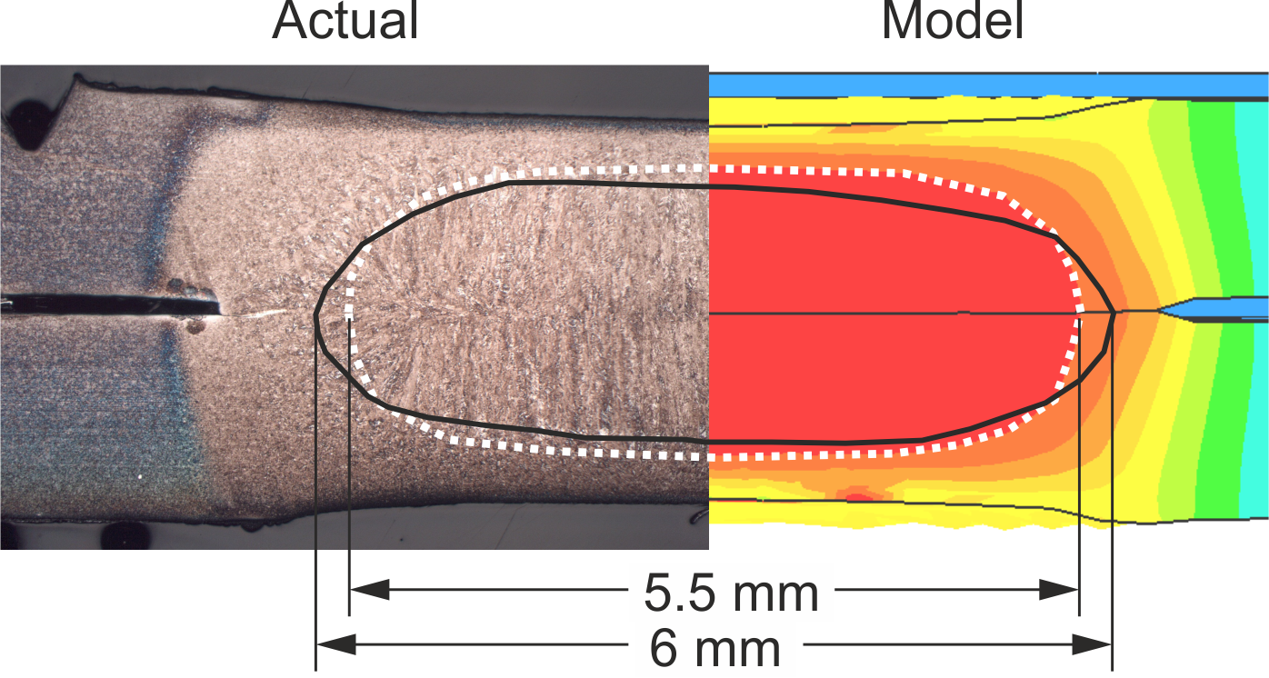
Finally, a metallographic cross-section shows whether the nugget size and -shape matches the experiment. The graphic shows a comparison between an actual and simulated cross section with a very small deviation of 0.5 mm in the diameter. As with the temperature measurements, a small deviation is not cause for concern. The experimental measurements also exhibit scatter, and there are a couple of simplifications in the model that will reduce the accuracy but still allow for fast calculation and good evaluation of trends.

Figure 3: Comparison of experimental and virtual cross-sections.F-23
After validation, consider conducting weldability investigations with the model. Try creating virtual force / current maps and the resulting nugget diameter to generate first guesses for experimental trials. We can also gain a feeling how the quality of each weld is affected by changes in coatings or by heated electrodes when we vary the boundary conditions for contact resistance and electrode cooling. The investigation of large spot-welded assemblies is possible for part fit-up and secondary effects such as shunting. Finally, the in-depth data on temperature flow and mechanical stresses is available for research-oriented investigations, cracking and joint strength impacts.
Note: The work represented in this article is a part a study of Liquid Metal Embrittlement (LME), commissioned by WorldAutoSteel. You can download the free report on the results of the LME study, including how this modelling was used to verify physical tests, from the WorldAutoSteel website.
RSW Modelling and Performance
This article summarizes the findings of a paper entitled, “Prediction of Spot Weld Failure in Automotive Steels,”L-48 authored by J. H. Lim and J.W. Ha, POSCO, as presented at the 12th European LS-DYNA Conference, Koblenz, 2019.
To better predict car crashworthiness it is important to have an accurate prediction of spot weld failure. A new approach for prediction of resistance spot weld failure was proposed by POSCO researchers. This model considers the interaction of normal and bending components and calculating the stress by dividing the load by the area of plug fracture.
Background
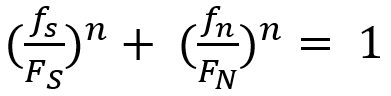
Lee, et al.L-49 developed a model to predict spot welding failure under combined loading conditions using the following equation, based upon experimental results .
|
Equation 1 |
Where FS and FN are shear and normal failure load, respectively, and n is a shape parameter.
Later, Wung and coworkersW-38 developed a model to predict the failure mode based upon the normal load, shear load, bending and torsion as shown in Equation 2.
 |
Equation 2 |
Here, FS, FN ,Mb and Mt are normal failure load, shear failure load, failure moment and failure torsion of spot weld, respectively. α, β, γ and μ are shape parameters.
Seeger et al.S-106 proposed a model for failure criterion that describes a 3D polynomial failure surface. Spot weld failure occurs if the sum of the components of the normal, bending and shear stresses are above the surface, as shown in the Figure 1.
Figure 1: Spot weld failure model proposed by Seeger et al.S-106
The failure criterion can be expressed via Equation 3.
 |
Equation 3 |
Here, σN , σB , and τ are normal, bending and shear stress of the spot weld, respectively. And nN, nB and nc are the shape parameters. Toyota Motor CorporationL-50 has developed the stress-based failure model as shown in Equation 4.
 |
Equation 4 |
Hybrid Method to Determine Coefficients for Failure Models
This work used a unique hybrid method to determine the failure coefficients for modeling. The hybrid procedure steps are as follows:
- Failure tests are performed with respect to loading conditions.
- Finite element simulations are performed for each experiment.
- Based on the failure loads obtained in each test, the instant of onset of spot weld failure is determined. Failure loads are extracted comparing experiments with simulations.
- Post processing of those simulations gives the failure load components acting on spot welds such as normal, shear and bending loads.
These failure load components are plotted on the plane consisting of normal, shear and bending axes.
The hybrid method described above is shown in Figure 2.L-48
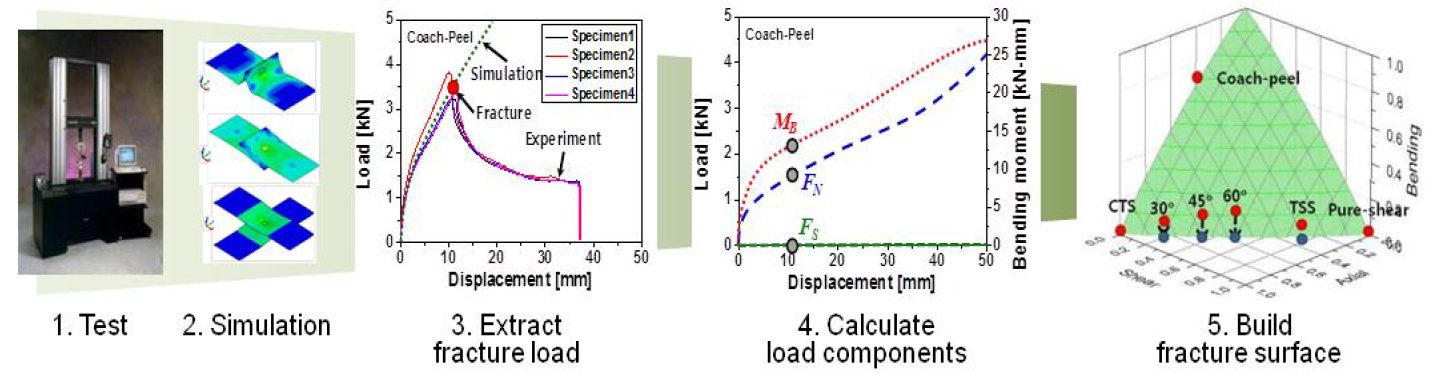
Figure 2: Hybrid method to obtain the failure load with respect to test conditions.L-48
New Spot Weld Failure Model
The new proposed spot weld failure model in this paper considers only plug fracture mode as a normal spot weld failure. Secondly normal and bending components considered to be dependent upon each other. Stress generated by normal and bending components is shear, and shear component generates normal stress. Lastly authors have used πdt to calculate the area of stress instead of πd2/4. The final expression is shown in the Equation 5.
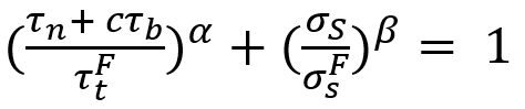 |
Equation 5 |
Here τn is the shear stress by normal load components, σS is the normal stress due to shear load component. And  ,
,  , c, α and β are coefficients.
This work included verification experiments of 42 kinds of homogenous steel stack-ups and 23 heterogeneous stack-ups. The strength levels of the steels used was between 270 MPa and 1500 MPa, and thickness between 0.55 mm and 2.3 mm. These experiments were used to evaluate the model and compare the results to the Wung model.
Conclusions
Overall, this new model considers interaction between normal and bending components as they have the same loading direction and plane. The current developed model was compared with the Wung model described above and has shown better results with a desirable error, especially for asymmetric material and thickness.
Simulation
Evaluating sheet metal formability using computer software has been in common industrial use for more than two decades. The current sheet metal forming programs are part of the transition to virtual manufacturing that includes analysis of casting solidification and rolling at the metal production facility, welding, moulding of sheet/fiber composites, automation, and other manufacturing processes. Computer simulation of sheet metal forming is known by several terms, including computerized forming process development and computerized die tryout.
Many highly developed software programs closely replicate the physical press shop forming of sheet metal stampings. These programs have proven to be accurate in predictions of blank movement, strains, thinning within the blank, wrinkles, buckles, and global formability concerns of necking strains and forming severity as defined by conventional forming limit curves. Accurate prediction of local formability related failures such as cut edge expansion is more challenging due to modeling of the production process influence as opposed to the ideal laboratory edge. Prediction of springback generally provides helpful results in understanding the trends and effects. The quality of springback predictions vary with the specific stamping geometry, the selected metal grade, the input information, and user experience, as discussed in Simulation Inputs.
Virtual forming-process development is ideally suited to the needs of current and potential users of AHSS grades. A full range of analysis capabilities is available to evaluate AHSS behavior in a new stamping. These programs allow rapid “what-if” scenarios to explore the impacts of different grades of AHSS, alternative processing, or even design optimization. A Design of Experiments on actual tooling in a physical press shop is limited to only a few variables and may be subject to noise variables clouding the results. In the virtual press shop, changing variables is done with a stroke of the keyboard, and is far easier to undo than permanent changes to the tooling.
Virtual die tryout has numerous advantages, allowing for assessing the viability of part, process, and die design all before cutting the first hard die. Addressing problems before costly and time-consuming die construction starts leads to improved quality and a better use of resources.
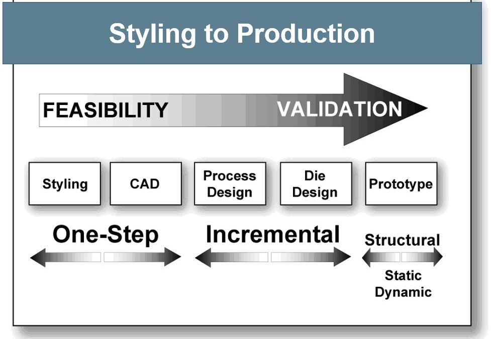
The type of software used depends on the goals and available information at each stage of the process, shown in Figure 1. At the beginning of the styling to production cycle, feasibility – whether the stamping can even be manufactured – is the key question. With only the 3D CAD file of the final part and material properties, One-Step or inverse codes can rapidly ascertain strain along section lines, thinning, forming severity, trim line-to-blank, hot spots, blank contour, and other key information. This approach takes the finished part geometry and unfolds that shape to generate a starting blank, calculating the strain between the two shapes (formed vs. flat). Since it starts with the finished geometry rather than the blank, the process is the inverse of reality. All deformation takes place in a single step, or one step, leading to the description of a one step inverse code. Although this takes reduced computing time, only some simulation packages allow incorporation of the forming process, tooling geometry, and the changes in metal properties associated with deformation.
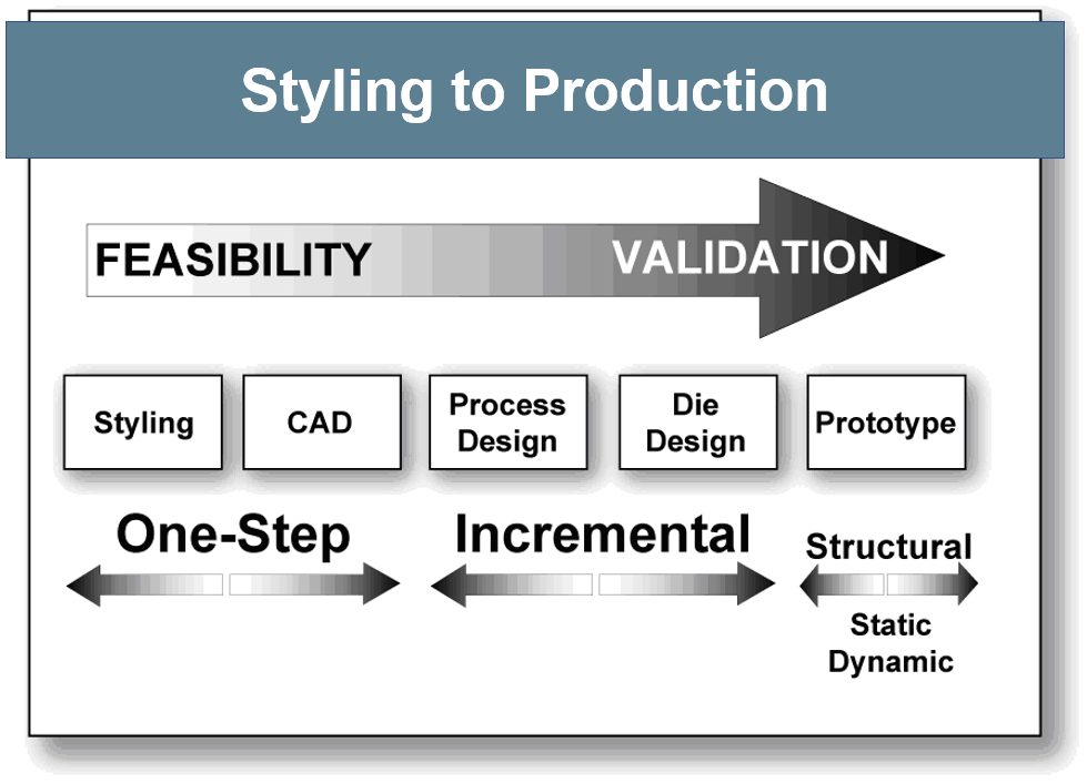
Figure 1: Software types change during processing stage.
Achieving more accurate results involves incremental simulation, where the virtual forming process attempts to replicate reality. This approach models the tools (punch, die, and blankholder) and process parameters (like the blankholder forces, blank shape, and bead geometry, location and restraining forces). Each increment, or time-step, reflects the sheet metal deformation at a different position of the press stroke. Subsequent increments rely on the output from the prior increments. As the quality of the inputs increase, so does the precision of the results.
During selection of process and die design parameters, software evaluates how each new input affects the strains and blank movement (including wrinkles and splits), and generates a press-loading curve. The analysis creates a visual record of the blank deformation into the final part through a transparent die. Each frame of the video is equivalent to an incremental hit or breakdown stamping. Problem areas or defects in the final increment of forming can be traced backwards through the forming stages to the initiation of the problem, allowing problems to be addressed when before they even occur. Some software packages allow analysis of multi-stage forming, such as progressive dies, transfer presses, or tandem presses. This virtual environment also shows the effects of trimming and other offal removal on dimensional precision and springback.
AHSS grades are suited for load bearing or crash-sensitive applications, and forming simulation helps to optimize performance. Previously, the static and dynamic capabilities of part and assembly designs were analyzed using CAD-generated stamping designs with inputs of initial sheet thickness and as-received yield strength. Often the tests results from real parts did not agree with these early analyses because the effects from forming were not incorporated. State-of-the-art applications now model the forming operation first, allowing for local thinning and work hardening to occur. That point-to-point sheet thickness and strength levels are mapped to the crash simulation inputs, resulting in crash models nearly identical to physical test outputs. Correcting deficiencies of the virtual parts by tool, process, or even part design occurs before tool construction has even begun.
Many simulation packages can evaluate the performance of AHSS grades in many forming environments. A simple constitutive equation with a single n-value sufficiently approximated the stress-strain response of older grades. The n-value of AHSS grades changes with strain, so when simulating AHSS grades, input the full stress-strain curve instead of choosing just one n-value. However, this capability may not be present in some proprietary industrial and university software. Use caution when using these programs to analyze AHSS stampings.
Today’s AHSS grades are not the commodities of yesteryear, but instead are highly engineered products unique to the production equipment and processing route chosen by the steelmaker. Although many companies may be capable of meeting the minimum and maximum mechanical properties associated with a specific grade, different suppliers may take up a different portion of the acceptable window. Working with your production steel supplier helps ensure you are using company-specific forming data.
Also remember that there are multiple products associated with a targeted tensile strength. For example, not only are there different families of 980 MPa minimum tensile strength steels (like dual phase, TRIP, and Q&P), but within each family there are multiple options. A grade designated as “DP980” may have enhanced global formability as measured with total elongation, enhanced local formability as measured in a hole expansion test, or have a balance between those properties. The associated material card for simulation will be different, and use of the incorrect card in development could lead to an under-engineered process when attempting to run with production steel.
Optimization Measures Applicable To Higher Strength Grades
- Simulation-driven compensation: Predict springback trends using metal forming simulation tools and apply geometric compensation to tooling surfaces based on sectional springback analysis.
- Process parameter optimization: Adjust blank holder force, drawbead resistance, and forming angles to balance material flow and reduce stress concentration.
- Post-forming correction: Add restriking or calibration processes to mitigate residual springback.
- Tooling design enhancements: Incorporate friction-reducing coatings and optimize mold geometry (e.g., increased draft angles) to control metal flow.
Key Points
- A virtual tryout evaluates the stamping and die design, and can detail areas of severe forming, buckles, excessive blank movement, and other undesirable deformation before starting tool construction.
- Evaluating alternative “what-if” scenarios in a virtual environment is faster and more efficient than grinding and welding on physical tooling, and mistakes have no permanent impact.
- Design of Experiments (DOE) studies are challenging to do in the physical press shop. The large number input changes required by the process makes it difficult to attribute changes to the intended variables tested or to some noise factor. Simulation allows for easier and faster evaluations when changing one or more parameters.
- AHSS grades change properties when deformed under different forming conditions. Forming simulation captures these changes to show how the final product will react.
- Observing the sheet metal transition from a flat blank to the engineered stamping in a transparent die is a valuable troubleshooting tool provided by virtual forming.
- Simulation codes accurately capture blank motion, thinning strains within the body of the stamping, and other global formability issues like severity compared with the conventional forming limit curve. However, prediction of local formability concerns like sheared edge stretchability is lacking due to the challenges of capturing all the effects related to creating that cut edge.
- The virtual forming codes do not accurately predict springback or the success of springback correction procedures because of the lack of pertinent data within a basic material card combined with the lack of accurate data everywhere in the stamping during the entire forming operation. However, users report reduction in recuts of the die from 12 or more to three or four based on information from the code.
A well-defined material card and accurate descriptions of metal flow throughout the stamping are critical for precise springback predictions, as discussed in the section on Simulation Inputs. Lacking that, many simulation packages can at least provide guidance on the trends which may help guide springback countermeasures.