Blog, RSW Modelling and Performance
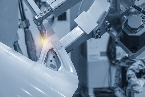
Modern car bodies today are made of increasing volumes of Advanced High-Strength Steels (AHSS), the superb performance of which facilitates lightweighting concepts (see Figure 1). To join the different parts of a car body and create the crash structure, the components are usually welded to achieve a reliable connection. The most prominent welding process in automotive production is resistance spot welding. It is known for its great robustness, and easily applicable in fully automated production lines.
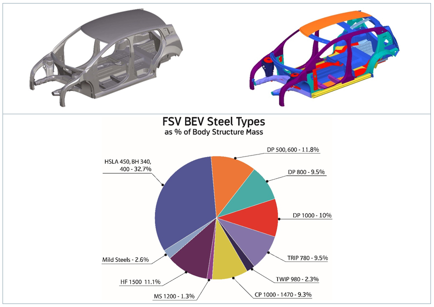
Figure 1: AHSS Content in Modern Car Body.W-7
There are, however, challenges to be met to guarantee a high-quality joint when the boundary conditions change, for example, when new material grades are introduced. Interaction of a liquefied zinc coating and a steel substrate can lead to small surface cracks during resistance spot welding of current AHSS, as shown in Figure 2. This so-called liquid metal embrittlement (LME) cracking is mainly governed by grain boundary penetration with zinc, and tensile stresses. The latter may be induced by various sources during the manufacturing process, especially under ‘rough’ industrial conditions. But currently, there is a lack of knowledge, regarding what is ‘rough’, and what conditions may still be tolerable.
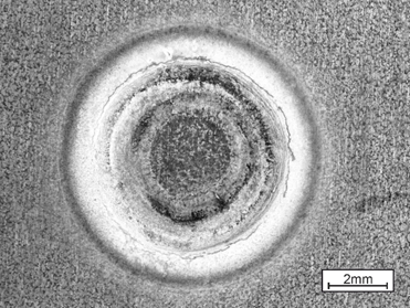
Figure 2: Top View of LME-Afflicted Spot Weld.
The material-specific amount of tensile stresses necessary for LME enforcement can be determined by the experimental procedure ‘welding under external load’. The idea of this method, which is commonly used for comparing cracking susceptibilities of different materials to each other, is to apply increasing levels of tensile stresses to a sample during the welding process and monitor the reaction. Figure 3 shows the corresponding experimental setup.

Figure 3: Welding under external load setup.L-51
However, the known externally applied stresses are not exclusively responsible for LME, but also the welding process itself, which puts both thermally and mechanically induced stresses/strains on the sample. Here, the conventional measuring techniques fail. A numerical reproduction of the experiment grants access to the temperature, stress and strain fields present during the procedure, providing insights on the formation of LME. The electro-thermomechanical simulation model is described in detail in Modelling RSW of AHSS. It is used to simulate the welding under external load procedure (see Figure 4).
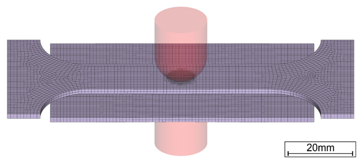
Figure 4: Simulation Model of Welding Under External Load.
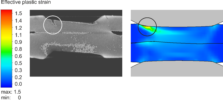
The videos that can be found in the link above show the corresponding temperature and plastic strain fields. As heat dissipates quickly through the water-cooled electrode, a temperature gradient towards the adjacent areas and a local temperature maximum on the surface forms. The plastic strains accumulate mainly at the electrode indentation area. The simulated strain field shows a local maximum of plastic deformation at the left edge of the electrode indentation, amplified by the externally applied stresses and the boundary conditions implied by the procedure. This area correlates with experimentally observed LME cracking sites and paths as shown in Figure 5.
The simulation shows that significant plastic strains are present during welding. When external stresses (in reality e.g. due to poor part fit-up or distorted parts) contribute to the already high load, LME cracking becomes more likely. The numerical simulation model facilitates the determination of material-specific safety limits regarding LME cracking. Parameter variations and their effects on the LME susceptibility can easily be investigated by use of the model, enabling the user to develop strict processing protocols to reduce the likelihood of LME. Finally, these experimental procedures can be adapted to other high-strength materials, to aid their application understanding and industrial set-up conditions.
Figure 5: LME Cracks in Cross Section View at Highly Strained Locations.
For more information on this topic, see the paper, co-authored by Fraunhofer and LWF Paderborn, documented in Citation F-23. You may also download the full report documenting the WorldAutoSteel LME project for which this work was conducted.
Blog, main-blog, RSW Modelling and Performance
Modelling resistance spot welding can help to understand the process and drive innovation by asking the right questions and giving new viewpoints outside of limited experimental trials. The models can calculate industrial-scale automotive assemblies and allow visualization of the highly dynamic interplay between mechanical forces, electrical currents and thermal flow during welding. Applications of such models allow efficient weldability tests necessary for new material-thickness combinations, thus well-suited for applications involving Advanced High -Strength Steels (AHSS).
Virtual resistance spot weld tests can narrow down the parameter space and reduce the amount of experiments, material consumed as well as personnel- and machine- time. They can also highlight necessary process modifications, for example the greater electrode force required by AHSS, or the impact of hold times and nugget geometry. Other applications are the evaluation of whole-part distortion to ensure good part-clearance and the investigation of stress, strain and temperature as they occur during welding. This more research-focused application is useful to study phenomena arising around the weld such as the formation of unwanted phases or cracks.
Modern Finite-Element resistance spot welding models account for electric heating, mechanical forces and heat flow into the surrounding part and the electrodes. The video shows the simulated temperature in a cross-section for two 1.5 mm DP1000 sheets:
First, the electrodes close and then heat starts to form due to the electric current flow and agglomerates over time. The dark-red area around the sheet-sheet interface represents the molten zone, where the nugget forms after cooling. While the simulated temperature field looks plausible at first glance, the question is how to make sure that the model calculates the physically correct results. To ensure that the simulation is reliable, the user needs to understand how it works and needs to validate the simulation results against experimental tests. In this text, we will discuss which inputs and tests are needed for a basic resistance spot welding model.
At the base of the simulation stands an electro-thermomechanical resistance spot welding model. Today, there are several Finite Element software producers offering pre-made models that facilitate the input and interpretation of the data. First tests in a new software should be conducted with as many known variables as possible, i.e., a commonly used material, a weld with a lot of experimental data available etc.
As first input, a reliable material data set is required for all involved sheets. The data set must include thermal conductivity and capacity, mechanical properties like Young’s modulus, tensile strength, plastic flow behavior and the thermal expansion coefficient, as well as the electrical conductivity. As the material properties change drastically with temperature, temperature dependent data is necessary at least until 800°C. For more commonly used steels, high quality data sets are usually available in the literature or in software databases. For special materials, values for a different material of the same class can be scaled to the respective strength levels. In any case, a few tests should be conducted to make sure that the given material matches the data set. The next Figure shows an exemplary material data set for a DP1000. Most of the values were measured for a DP600 and scaled, but the changes for the thermal and electrical properties within a material class are usually small.
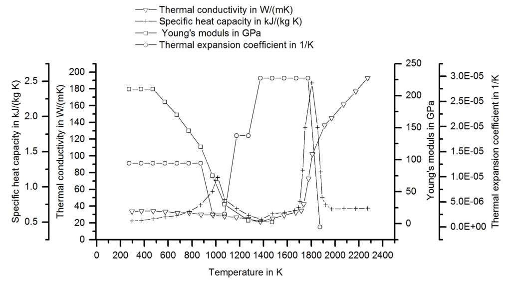
Figure 1: Material Data set for a DP1000.S-73
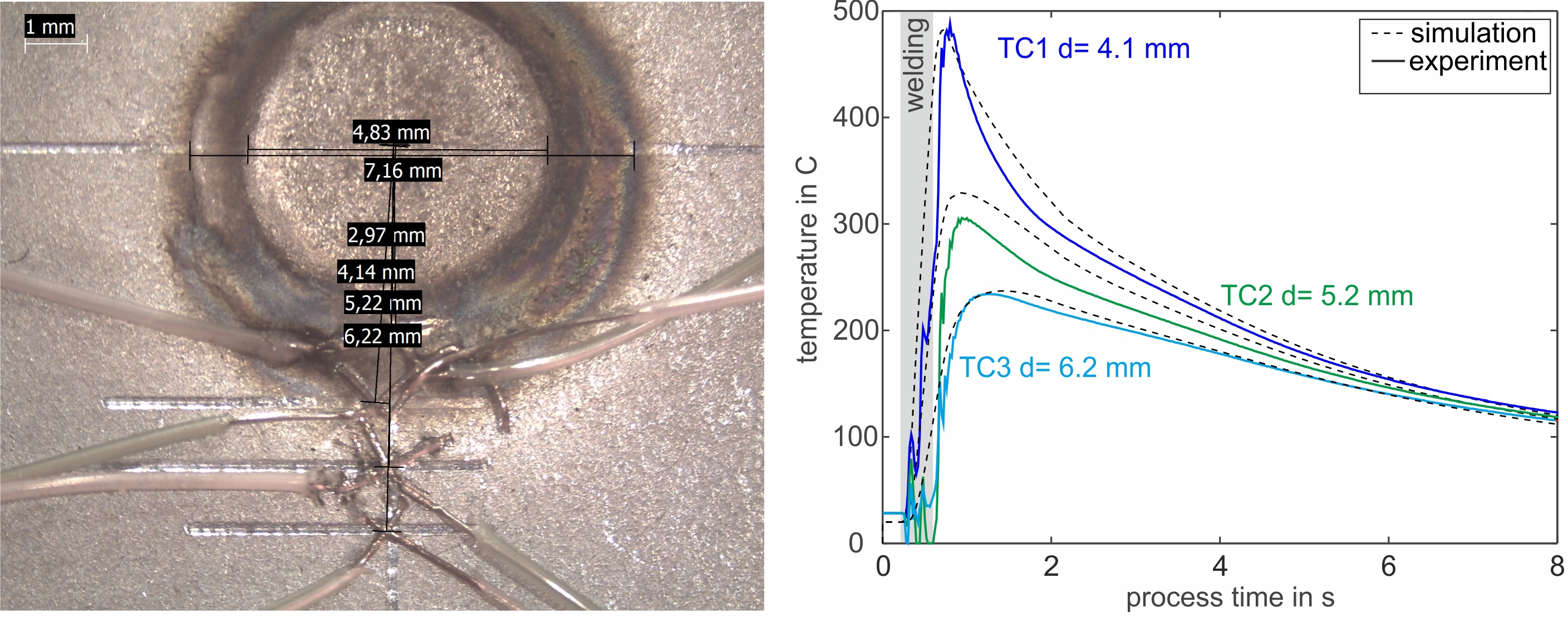
Next, meaningful boundary conditions must be chosen and validated against experiments. These include both the electrode cooling and the electrical contact resistance. To set up the thermal flow into the electrode, temperature measurements on the surface are common. In the following picture, a measurement with thermocouples during welding and the corresponding result is shown. By adjusting the thermal boundary in the model, the simulated temperatures are adjusted until a good match between simulation and experiment is visible. This calibration needs to be conducted only once when the model is established because the thermal boundary remains relatively constant for different materials and coatings.
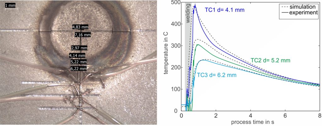
Figure 2: Temperature measurement with thermocouples during welding and the results. The simulated temperature development is compared to the experimental curve and can be adjusted via the boundary conditions.F-23
The second boundary condition is the electrical contact resistance and it is strongly dependent on the coating, the surface quality and the electrode force. It needs to be determined experimentally for every new coating and for as many material thickness combinations as possible. In the measuring protocol, a reference test eliminates the bulk material resistance and allows for the determination of the contact resistances using a µOhm-capable digital multimeter.
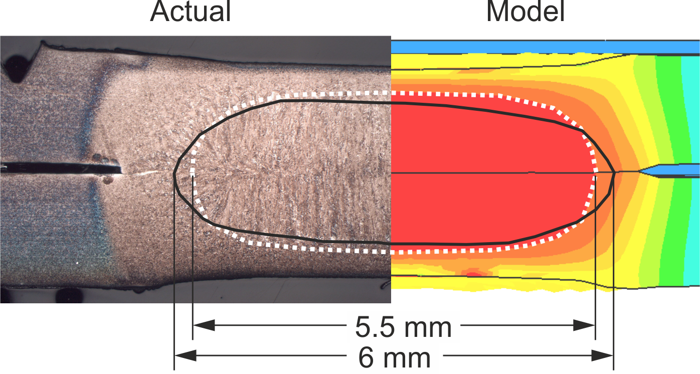
Finally, a metallographic cross-section shows whether the nugget size and -shape matches the experiment. The graphic shows a comparison between an actual and simulated cross section with a very small deviation of 0.5 mm in the diameter. As with the temperature measurements, a small deviation is not cause for concern. The experimental measurements also exhibit scatter, and there are a couple of simplifications in the model that will reduce the accuracy but still allow for fast calculation and good evaluation of trends.

Figure 3: Comparison of experimental and virtual cross-sections.F-23
After validation, consider conducting weldability investigations with the model. Try creating virtual force / current maps and the resulting nugget diameter to generate first guesses for experimental trials. We can also gain a feeling how the quality of each weld is affected by changes in coatings or by heated electrodes when we vary the boundary conditions for contact resistance and electrode cooling. The investigation of large spot-welded assemblies is possible for part fit-up and secondary effects such as shunting. Finally, the in-depth data on temperature flow and mechanical stresses is available for research-oriented investigations, cracking and joint strength impacts.
Note: The work represented in this article is a part a study of Liquid Metal Embrittlement (LME), commissioned by WorldAutoSteel. You can download the free report on the results of the LME study, including how this modelling was used to verify physical tests, from the WorldAutoSteel website.
RSW Modelling and Performance
This article summarizes the findings of a paper entitled, “Prediction of Spot Weld Failure in Automotive Steels,”L-48 authored by J. H. Lim and J.W. Ha, POSCO, as presented at the 12th European LS-DYNA Conference, Koblenz, 2019.
To better predict car crashworthiness it is important to have an accurate prediction of spot weld failure. A new approach for prediction of resistance spot weld failure was proposed by POSCO researchers. This model considers the interaction of normal and bending components and calculating the stress by dividing the load by the area of plug fracture.
Background
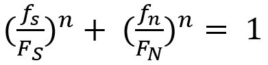
Lee, et al.L-49 developed a model to predict spot welding failure under combined loading conditions using the following equation, based upon experimental results .
|
Equation 1 |
Where FS and FN are shear and normal failure load, respectively, and n is a shape parameter.
Later, Wung and coworkersW-38 developed a model to predict the failure mode based upon the normal load, shear load, bending and torsion as shown in Equation 2.
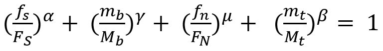 |
Equation 2 |
Here, FS, FN ,Mb and Mt are normal failure load, shear failure load, failure moment and failure torsion of spot weld, respectively. α, β, γ and μ are shape parameters.
Seeger et al.S-106 proposed a model for failure criterion that describes a 3D polynomial failure surface. Spot weld failure occurs if the sum of the components of the normal, bending and shear stresses are above the surface, as shown in the Figure 1.
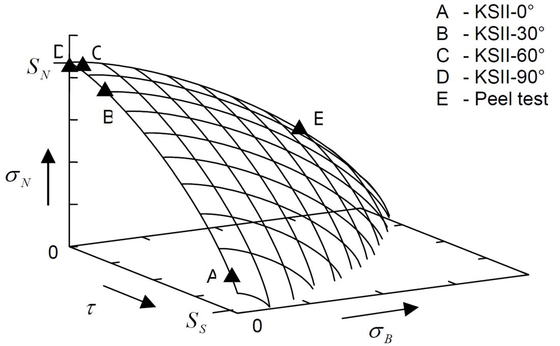
Figure 1: Spot weld failure model proposed by Seeger et al.S-106
The failure criterion can be expressed via Equation 3.
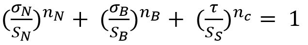 |
Equation 3 |
Here, σN , σB , and τ are normal, bending and shear stress of the spot weld, respectively. And nN, nB and nc are the shape parameters. Toyota Motor CorporationL-50 has developed the stress-based failure model as shown in Equation 4.
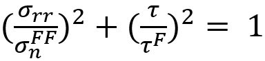 |
Equation 4 |
Hybrid Method to Determine Coefficients for Failure Models
This work used a unique hybrid method to determine the failure coefficients for modeling. The hybrid procedure steps are as follows:
- Failure tests are performed with respect to loading conditions.
- Finite element simulations are performed for each experiment.
- Based on the failure loads obtained in each test, the instant of onset of spot weld failure is determined. Failure loads are extracted comparing experiments with simulations.
- Post processing of those simulations gives the failure load components acting on spot welds such as normal, shear and bending loads.
These failure load components are plotted on the plane consisting of normal, shear and bending axes.
The hybrid method described above is shown in Figure 2.L-48
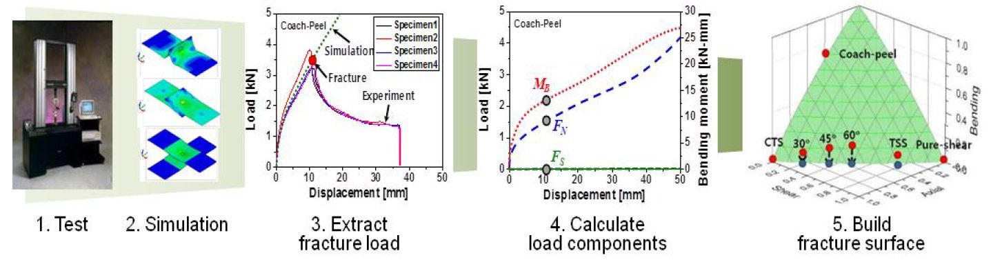
Figure 2: Hybrid method to obtain the failure load with respect to test conditions.L-48
New Spot Weld Failure Model
The new proposed spot weld failure model in this paper considers only plug fracture mode as a normal spot weld failure. Secondly normal and bending components considered to be dependent upon each other. Stress generated by normal and bending components is shear, and shear component generates normal stress. Lastly authors have used πdt to calculate the area of stress instead of πd2/4. The final expression is shown in the Equation 5.
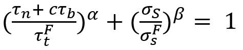 |
Equation 5 |
Here τn is the shear stress by normal load components, σS is the normal stress due to shear load component. And  ,
,  , c, α and β are coefficients.
This work included verification experiments of 42 kinds of homogenous steel stack-ups and 23 heterogeneous stack-ups. The strength levels of the steels used was between 270 MPa and 1500 MPa, and thickness between 0.55 mm and 2.3 mm. These experiments were used to evaluate the model and compare the results to the Wung model.
Conclusions
Overall, this new model considers interaction between normal and bending components as they have the same loading direction and plane. The current developed model was compared with the Wung model described above and has shown better results with a desirable error, especially for asymmetric material and thickness.
RSW of Dissimilar Steel
This article is the summary of a paper entitled, “HAZ Softening of RSW of 3T Dissimilar Steel Stack-up”, Y. Lu., et al.L-15
Electromechanical Model
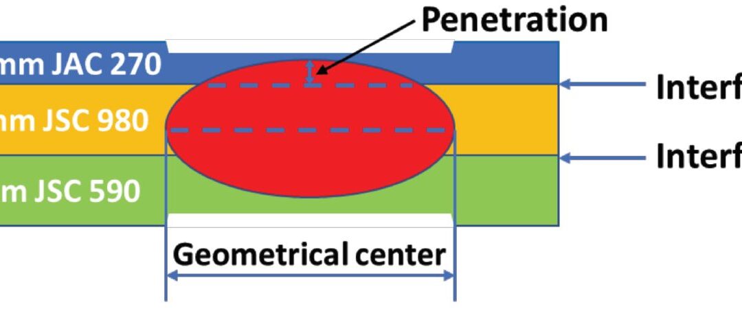
The study discusses the development of a 3D fully coupled thermo-electromechanical model for RSW of a three sheet (3T) stack-up of dissimilar steels. Figure 1 schematically shows the stack-up used in the study. The stack-up chosen is representative of the complex stack-ups used in BIW. Table 1 summarizes the nominal compositions of the three steels labeled in Figure 1.
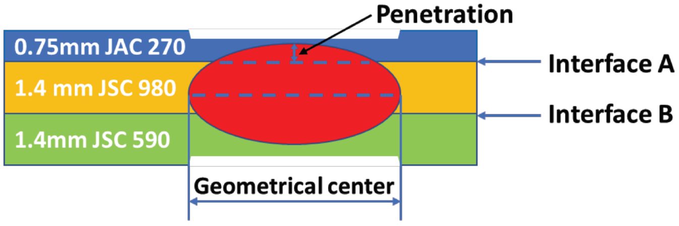
Figure 1: Schematics of the 3T stack-up of 0.75-mm-thick JAC 270/1.4-mm-thick JSC 980/1.4-mm-thick JSC 590 steels.L-15
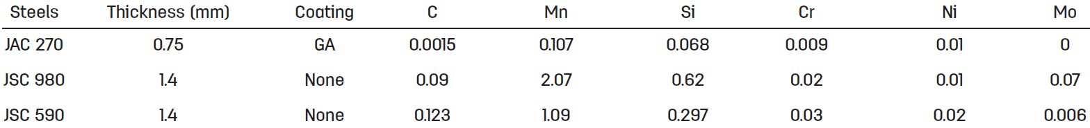
Table 1: Nominal Composition of Steels.L-15
JAC270 is a cold rolled Mild steel with a galvanneal coating having a minimum tensile strength of 270 MPa. JSC590 and JSC980 are bare cold rolled Dual Phase steels with a minimum tensile strength of 590 MPa and 980 MPa, respectively.
The electrodes used were CuZr dome-radius electrodes with a surface diameter of 6 mm. The welding parameters are listed in Table 2.
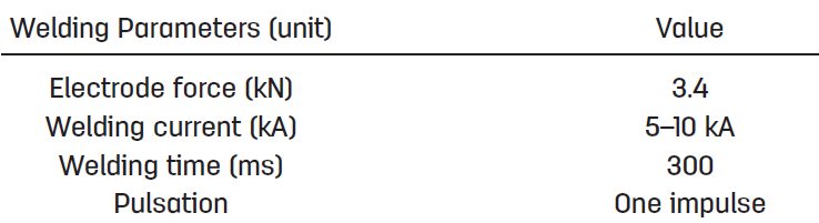
Table 2: Welding Parameters for Resistance Spot Welding of 3T Stack-Up of Steel Sheets.L-15
Figure 2 shows consistent nugget dimensions between simulation and experiment, supporting the validity of the RSW process model for 3T stack-up. The effect of welding current on nugget penetration into the thin sheet is similar to that on the nugget size. It increases rapidly at low welding current and saturates to 32% when the welding current is higher than 9 kA, as shown in Figure 2C.
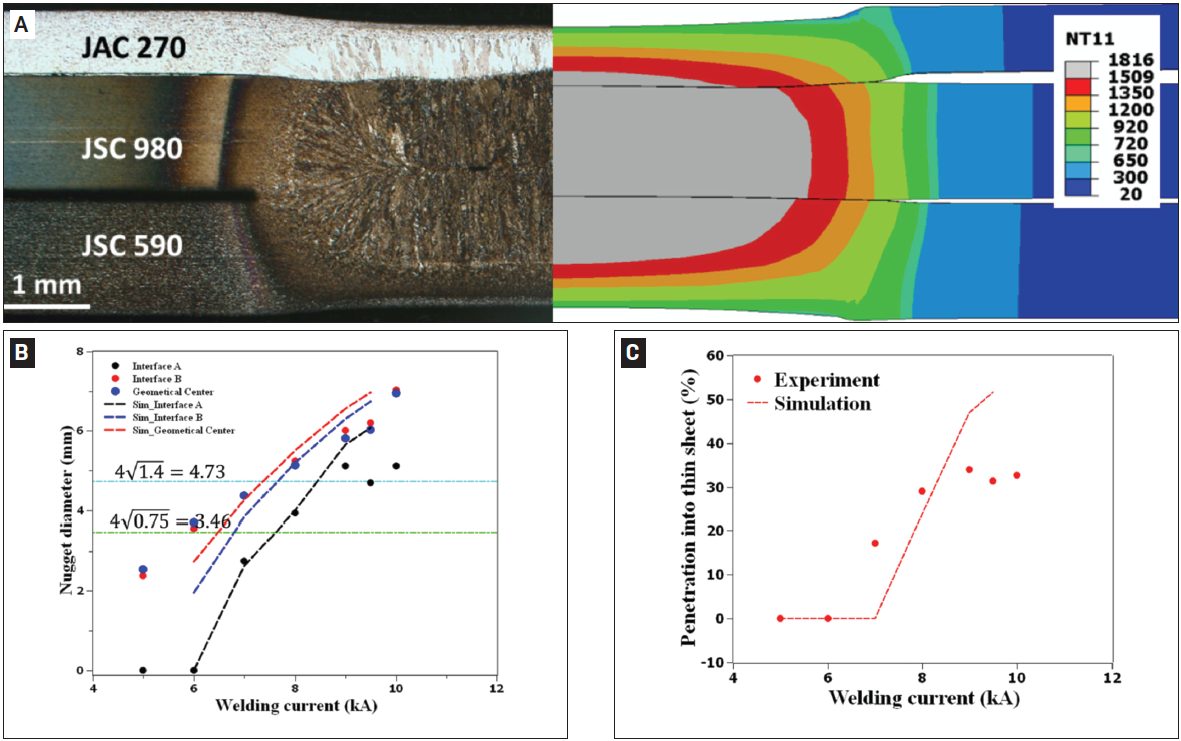
Figure 2: Comparison between experimental and simulated results: A) Nugget geometry at 8 kA; B) nugget diameters; C) nugget penetration into the thin sheet as a function of welding current. In Figure 2A, the simulated nugget geometry is represented by the distribution of peak temperature (in Celsius). The two horizontal lines in Figure 2B represent the minimal nugget diameter at Interfaces A and B calculated, according to AWS D8.1M: 2007, Specification for Automotive Weld Quality Resistance Spot Welding of Steel. Due to limited number of samples available for testing, the variability in nugget dimensions at each welding current was not measuredL-15.
The results for nugget formation during RSW of the 3T stack-up are show in Figures 3-5. Figure 2 shows that, at the start of welding, the contact pressure at interface A (thin/thick) has a higher peak and drops more quickly along the radial direction than that at interface B (thick/thick). Due to the more localized contact area (Figure 3), a high current density can be observed at interface A, as shown in Figure 4A. Additionally, due to the high current density at interface A, localized heating is generated at this interface, as shown in Figure 5A.
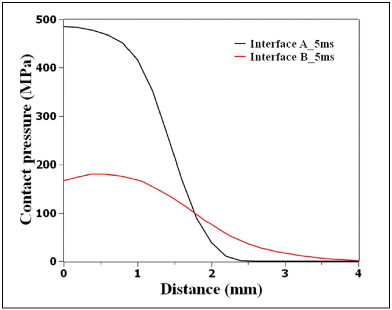
Figure 3: Calculated contact pressure distribution at interfaces A (thin/thick) and B (thick/thick) at a welding time of 5 ms, current of 8 kA, and electrode force of 3.4 L-15
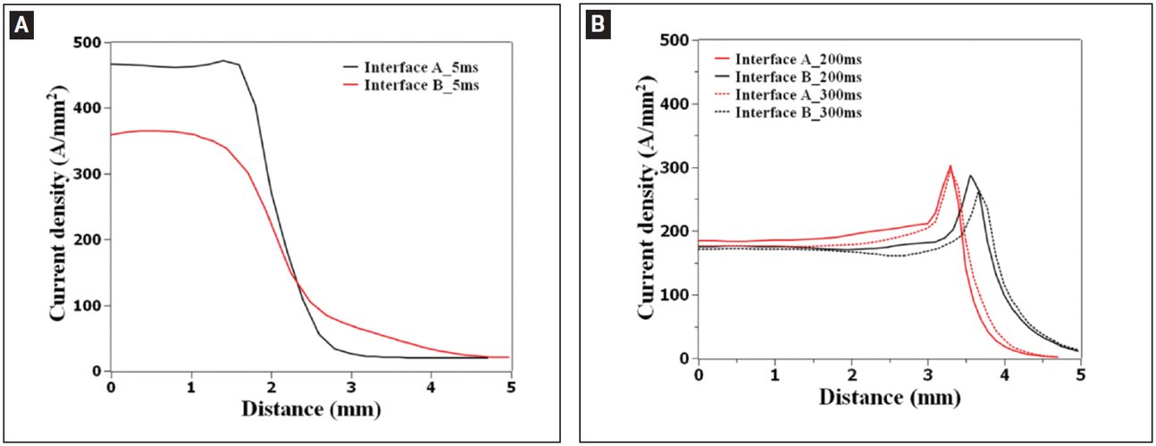
Figure 4: Calculated current density distribution at interfaces A (thin/thick) and B (thick/thick) at welding time of A — 5 ms; B — 200 and 300 ms.L-15
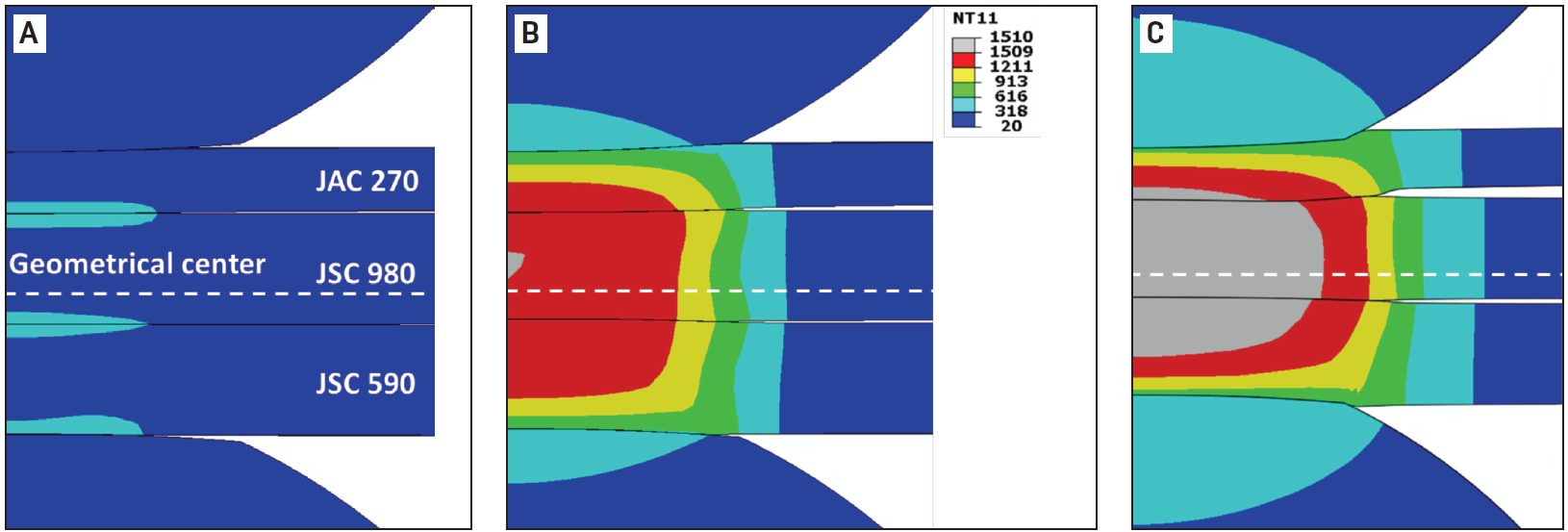
Figure 5: Temperature distribution during resistance spot welding of 3T stack-up at welding times of A) 5 ms; B) 102 ms; C) 300 ms. Welding current is 8 kA and electrode force is 3.4 kN. Calculated temperature is given in Celsius.L-15
As welding time increases, the contact area is expanded, resulting in a decrease of current density. The heat generation rate is shifted from interfaces to the bulk and the peak temperature occurs near the geometrical center of the stack-up.
Figure 6 illustrates that the predicted value corresponds well with the experimental data indicating a sound fitting to the isothermal tempering experimental data.
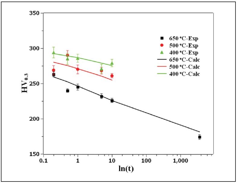
Figure 6: Comparison of the measured hardness with JMAK calculation showing the goodness of fit of the JSC 980 tempering kinetics parameters.L-15
Figure 7 shows the predicted hardness map of RSW 3T stack-up as well as the predicted and measured hardness profiles for JSC 980.
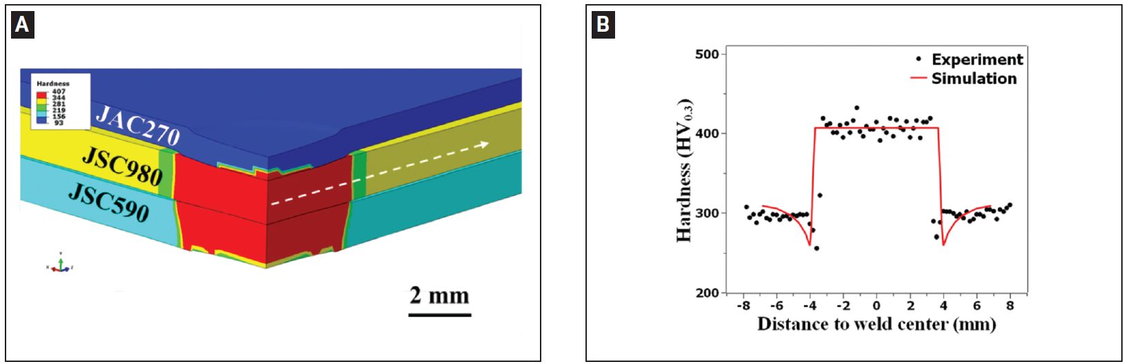
Figure 7: A) Predicted hardness map of resistance spot welded 3T stack-up; B) predicted and measured hardness profiles along the line marked in (A) for JSC 980.L-15
RSW Modelling and Performance
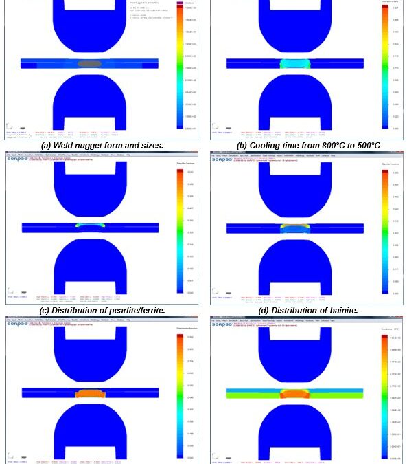
The advantages of numerical simulations for resistance welding are obvious for saving time and reducing costs in product developments and process optimizations. Today’s modeling techniques can predict temperature, microstructure, stress, and hardness distribution in the weld and Heat Affected Zone (HAZ) after welding. Commercial modeling software is available which considers material type, various current modes, machine characteristics, electrode geometry, etc. An example of process simulation results for spot welding of 0.8-mm DC 06 low-carbon steel to 1.2-mm DP 600 steel is shown in Figure 1. Obviously, this technique can apply to dissimilar thicknesses, material types, and geometries. Application of adhesives is also being used with these simulations. This simulation techniques are found to be very beneficial to predict vehicle crashworthiness as it can dramatically reduce the cost of crash evaluations.
You will find several articles in this section describing RSW modelling studies and procedures.
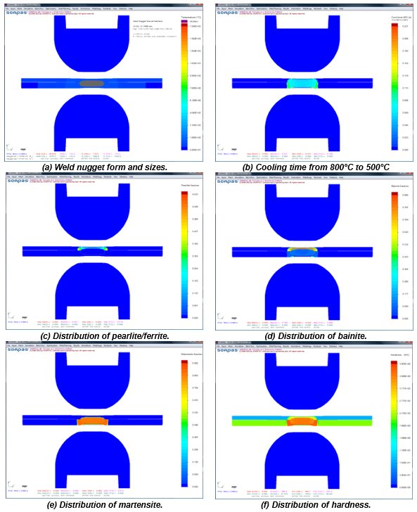
Figure 1: Simulation results with microstructures and hardness distribution for spot welding of 0.8-mm DC06 low-carbon steel to 1.2-mm DP 600 steel.Z-1