![Forming Limit Curves (FLC)]()
Formability
topofpage
If all stampings looked like a tensile dogbone and all deformation was in uniaxial tension, then a tensile test would be sufficient to characterize the formability of that metal. Obviously, engineered stampings are much more complex. Although a tensile test characterizes one specific strain path, a Forming Limit Curve (FLC) is necessary to have a map of strains indicating the onset of critical through-thickness necking for different linear strain paths. The strains which make up the FLC represent the limit of useful deformation. Calculations of safety margins are based on the FLC (Figure 1).

Figure 1: General graphical form of the Forming Limit Curve.E-2
Picturing a blank covered with circles helps visualize strain paths. After forming, the circles turn into ellipses, with the dimensions related to the major and minor strains. This forms the basis for Circle Grid Strain Analysis.
Generating Forming Limit Curves from Equations
Pioneering work by Keeler, Brazier, Goodwin and others contributed to the initial understanding of the shape of the Forming Limit Curve, with the classic equation for the lowest point on the FLC (termed FLC0) based on sheet thickness and n-value. Dr. Stuart Keeler was the Technical Editor of these AHSS Guidelines through Version 6.0, released in 2017.
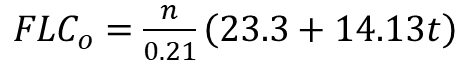 |
Equation 1 |
These studies generated the left hand side of the FLC as a line of constant thinning in true strain space, while the right hand side has a slope of +0.6, at least through minor (engineering) strains of 20%.
Evidence accumulated over many decades show that this approach to defining the Forming Limit Curve is sufficient for many applications of mild steels, conventional high strength steels, and some lower strength AHSS grades like CR340Y/590T-DP. However, this basic method is insufficient when it comes to creating the Forming Limit Curves for most AHSS grades and every other sheet metal alloy. Grades with significant amounts of retained austenite experience significant deviations from these simple estimates.H-23, S-61 In these cases, the FLC must be experimentally determined.
Additional studies found correlation with other properties including total elongation, tensile strength, and r-valueR-8, P-19, G-23, A-45, A-46, H-23 with some of these attempting to define the FLC by equations.
Experimental Determination of Forming Limit Curves
ASTM A-47 and ISO I-16 have published standards covering the creation of FLCs. Even within these standards, there are many nuances left for interpretation, primarily related to the precise definition of when a neck occurs and the associated limiting strains.
There are two steps in creating FLCs: Forming the samples and measuring the strains.
Forming sheet specimens of different widths uses either a hemispherical dome (Nakajima or Nakazima method N-14) or a flat-bottom punch (Marciniak method M-22) to generate different strain paths from which critical strains are determined. The two methods are not identical due to the different strain paths generated from the punch shape. These differences may not be significant for many lower strength and conventional High-Strength Steels, but may deviate from each other at higher strengths or with advanced microstructures. Figure 2 highlights samples formed with the Nakajima method.
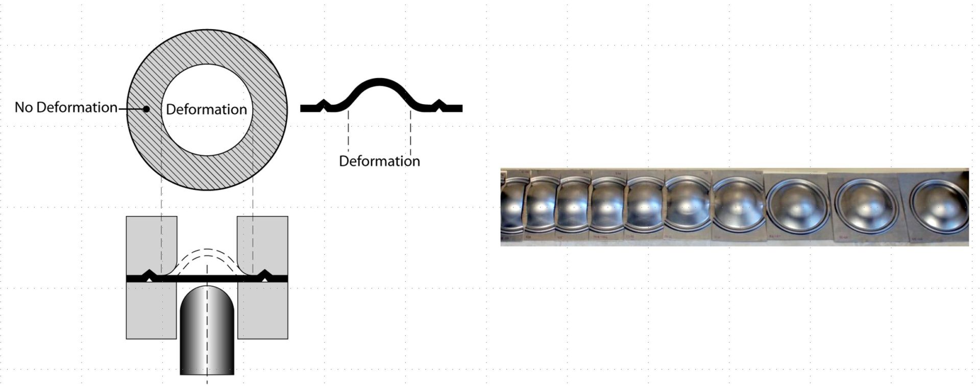
Figure 2: Forming limit curves can be created by deforming multiple samples of different widths. Narrow strips on the left allow metal to flow in from the unconstrained edges, creating a draw deformation mode leading to strains that plot on the left side of the FLC. Fully constrained samples, shown on the rightE-2, create a stretch deformation mode leading to strains that plot on the right side of the FLC.
Generally, strains are measured using one of two methods. The first approach involves covering the initially flat test samples with a grid pattern of circles, squares, or dots of known diameter and spacing to measure the strains associated with deformation. An alternate approach is based on Digital Image Correlation (DIC), where a camera tracks the movement of a random speckle pattern applied prior to forming.W-26, H-22, M-21 DIC methods are directly suited for use with stress-based FLCs.
Differences between Forming Limit Curves
and Forming Limit Diagrams
Often, the terms Forming Limit Curve (FLC) and Forming Limit Diagram (FLD) are used interchangeably. Perhaps a better way of categorizing is to define the components and what they encompass. This is somewhat of a simplification, since detailed interactions are known to occur.
- The Forming Limit Curve is a material parameter reflecting of the limiting strains resulting in necking failure as a function of strain path. It is a function of the metal grade, thickness, and sheet surface conditions, as well as the methods used during its creation (hemispherical/flat punch, test speed, temperature). It is applicable to any part shape.
- Deforming a flat sheet into an engineered stamping results in a formed surface with strains as a function of the forming conditions like local radii, lubrication, friction, and of course part geometry. These strains are essentially independent of the chosen metal grade and thickness. Plotting these strains allows for a relative assessment of which strains are higher than others, but no judgment can be made on “how high is too high?”
- The Forming Limit Diagram is a combination of the Forming Limit Curve (a material property) and the strains (reflecting part geometry and forming conditions). The FLD provides guidance on which areas of the formed part requires additional attention to achieve robust stamping conditions. Creating a subsequent FLD may be warranted when conditions change, since changes to the sheet metal properties (FLC) and the forming conditions (radii, lubrication, beads, blank size) will change the FLD, potentially affecting the conclusions.
Key Points
-
- Conventional Forming Limit Curves characterize necking failure only. Fractures at cut edges and tight bends may occur at strains lower than that suggested by the Forming Limit Curve.
- Differences in determination and interpretation of FLCs exist in different regions of the world.
- This system of FLCs commonly used for low strength and conventional HSLA is generally applicable to experimental FLCs obtained for DP steels for global formability.
- The left side of the FLC (negative minor strains) is in good agreement with experimental data for DP and TRIP steels. The left side depicts a constant thinning strain as a forming limit.
- Determination of FLCs for TRIP, MS, TWIP, and other special steels typically requires an experimental approach, since conventional simple equations do not accurately reflect the forming limits for these advanced microstructures.
Back to the Top
Formability
A Forming Limit Curve (FLC) is a map of strains indicating the onset of critical through-thickness necking for different linear strain paths. The FLC is dependent on the metal grade and the specific methods used in its creation. When paired with the strains generated during forming of an engineered part, the associated Forming Limit Diagram (FLD) provides guidance on which areas of the part might be prone to necking failures during production stamping conditions that replicate those used in the analysis.
Several methods are available to measure the strains on formed parts. The earliest method is known as Circle Grid Strain Analysis (CGSA), with Dr. Stuart Keeler as its primary evangelist for nearly 50 years. Dr. Keeler was the Technical Editor of these AHSS Guidelines through Version 6.0, released in 2017.
As the name suggests, a flat blank is covered with a grid of circles of precisely known diameter, typically applied by electrochemical etching. Forming turns the circles into ellipses, with the dimensions related to the major and minor strains. Conventional measurement occurs after forming, and involves a calibrated Mylar™ strip marked with gradations indicating the expansion or contraction relative to the initial circle diameter. Typically, these are viewed through magnifiers, making it easier to discern the critical dimensional differences. Techniques and caveats are highlighted in Citations S-59 and S-60.
Instead of circles, most camera-based measurement techniques for analysis after forming use a regular grid pattern of squares or dots. Forming turns the squares into rectangles, and the camera/computer measures the expansion or contraction of the nodes at the corners of the squares to determine the strains. Similarly, forming changes the regular dot pattern, allowing for calculation of the strains.
These approaches determine only the strains after forming, and are constrained to assume linear strain paths. An alternate approach based on Digital Image Correlation (DIC), where a camera tracks the movement of a random speckle pattern applied prior to forming,W-26, H-22, M-21 follows the strain evolution which occurs during forming and is not affected by non-linear strain paths.
Although DIC strain analysis is more accurate and informative, it is a higher-cost approach best suited for laboratory environments. Circle-grid, square-grid, and dot-grid strain analysis are all lower cost options and readily applied on the shop floor. Each of these in-plant techniques have different merits and challenges, including ease of use, accuracy, and cost.
![Forming Limit Curves (FLC)]()
FLC and FLD
Conventional Forming Limit Curves (FLCs) gained widespread industrial use since being introduced by Dr. Stuart Keeler in the 1960’s. Applications from feasibility analysis to stamping plant troubleshooting use these principles. The strain hardening exponent (n-value) and thickness are inputs into a shortcut to create the curve placement and shape, but this is applicable to only mild steels, conventional High-Strength Steels, and some Advanced High-Strength Steels. Furthermore, this shortcut is an approximation, coming from a best-fit curve generated from data points gathered over multiple grades.
A typical method used in creating most FLCs includes deforming samples of different widths with a 100 mm (4 inch) diameter hemispherical punch – known as the Nakajima method. An alternate approach uses a flat-bottom cylindrical punch, known as the Marciniak method (Figure 1). Independent of the punch shape used, generating FLCs involves measuring the strains resulting from deforming a blank to a formed shape. The conventional FLC plots major strain on the vertical axis against minor strain on the horizontal axis. This FLC applies only to in-plane stretching in linear strain paths, and assumes that there are no through-thickness stress or strain differences. Assessing bendability or cut edge ductility is not possible with this approach.
![Figure 1: Punch Shape Used to Create Forming Limit Curves Result in Through-Thickness Strain Differences Which Influence the Shape and Placement of The FLC [Reference 1]](https://ahssinsights.org/wp-content/uploads/2020/09/2.3.3.2-Fig1-Domes.svg)
Figure 1: Punch Shape Used to Create FLCs Result in Through-Thickness Strain Differences Which Influence the Shape and Placement of The FLC S-37
Figure 2 compares the FLCs generated by deforming DP980 with the three punch shapes highlighted in Figure 1. Note the higher strains associated with the 50 mm diameter hemispherical punch compared with the strains generated from the 100 mm diameter hemispherical punch. This punch curvature difference impacts the magnitude of the strains that develop through the thickness of the sheet. On samples deformed with a hemispherical punch, the selected strain measurement technique (circle/square grid analysis or Digital Image Correlation, for example) directly measures strains on the outer top surface only, with the middle and inner surface having progressively lower strains as a function of the R/T ratio. A punch or feature with small R/T leads to high strains on the outermost surface. Strains exceeding the FLC on only this outer surface will not lead to necks on the formed panel. Exceeding the FLC through the entire thickness – from the inner surface to the outer surface – must occur for the sample to show a neck.T-17
![Figure 2: FLCs of the same batch of DP980 Showing Dependence on Punch Shape and Curvature [References 1 and 3]](https://ahssinsights.org/wp-content/uploads/2020/09/2.3.3.2-Fig2-FLC-different.svg)
Figure 2: FLCs of the same batch of DP980 Showing Dependence on Punch Shape and Curvature.S-37, M-15
In addition to the through-thickness strain differences from the punch curvature, the metal flow differences resulting from the punch shapes leads to directional changes in the strain path taken by the deforming metal. A channel drawn part with a hat-shaped cross section in which there are no features like embossments is likely to have a linear strain path. Forming every other engineered stamped part geometry involves some degree of a non-linear strain path (NLSP).
The importance of strain path and deformation history comes from the changes in the forming limit that occur once metal deformation starts. The black curve in Figure 3 shows the FLC for an alloy generated in a conventional manner with as-received metal, assuming a linear strain path. The red curve results from testing the same metal that initially stretched to an equal-biaxial plastic pre-strain of 0.07. In this strain path, substantially less deformation can occur before reaching the forming limit. However, the strain path changes if the local part contour is different, and that strain path results in a different amount of subsequent deformation prior to necking. The magnitude and direction of the shift changes based on the strain and the orientation relative to the rolling direction. Citation S-38 highlights these curves and presents more examples of the effects of different strain paths. The important conclusion is that the amount of deformation that a metal is capable of withstanding prior to necking changes throughout the forming process and depends on the local part shape (among other variables), and cannot be discerned by using only the conventional strain based FLC.
![Figure 3: Experimental FLCs for a linear strain path (in black) and for a bilinear strain path after 0.07 strain in equal biaxial tension in strain space (in red) [Reference 4]](https://ahssinsights.org/wp-content/uploads/2020/09/2.3.3.2-Figure3-FLC-strainPath.svg)
Figure 3: Experimental FLCs for a linear strain path (in black) and for a bilinear strain path after 0.07 strain in equal biaxial tension in strain space (in red) S-38
Figure 4 shows the strain paths associated with the FLCs presented in Figure 2, with along with a magnified portion of one of the curves. This non-linearity is a characteristic of samples formed with a dome, associated with the sample wrapping around the punch during the initial contact and experiencing a combination of biaxial bending and stretching. Citation M-15 presents a method to correct for strain path effects.
![Figure 4: Strain Path for FLCs shown in Figure 2. A) 100mm diameter flat punch; B) 100mm diameter hemispherical punch; C) 50mm diameter hemispherical punch; and D) Magnified portion of one curve from Figure 4B showing the non-linearity of the strain path [References 1 and 3]](https://ahssinsights.org/wp-content/uploads/2020/09/2.3.3.2-Figure4-FLC-strainPath.svg)
Figure 4: Strain Path for FLCs shown in Figure 2. A) 100 mm diameter flat punch; B) 100 mm diameter hemispherical punch; C) 50 mm diameter hemispherical punch; and D) Magnified portion of one curve from Figure 4B showing the non-linearity of the strain path.S-37, M-15
Accounting for tool contact pressure is critical as well, since pressure through the sheet thickness suppresses the onset of necking. Applying this compensated FLC in simulation or in hands-on analysis parts analysis requires modification for the unique characteristics of each part, with appropriate adjustments for local curvature, contact pressure and deformation history. Citations S-37 and M-15 detail methods to compensate for the effects of strain path, curvature, and tool pressure. Figure 5 shows that after incorporating these corrections, the curves condense to one shape independent of the variables used.
![Figure 5: As-generated FLCs compared with FLCs after strain path, curvature, and tool contact pressure corrections [References 1 and 3]](https://ahssinsights.org/wp-content/uploads/2020/09/2.3.3.2_5.jpg)
Figure 5: As-generated FLCs compared with FLCs after strain path, curvature, and tool contact pressure corrections.S-37, M-15
In summary, FLCs generated from relatively similar simple tools are sensitive to small differences in R/T ratio, incorporation of tool contact pressure, and deviations from a linear strain path. By comparison, engineered stampings require substantially more complex tool shapes with differing degrees of curvature, tool contact pressure, and strain paths all within one part. These complex part shapes contribute to an even wider variation in the yield surface and hardening mechanisms important for simulation, and impacts predictions of formability, springback, and stress analysis.
A common requirement during tooling buyoff – where all strains need to be below the FLC by at least a certain amount called the safety margin – magnifies these challenges. AHSS grades already have low FLCs relative to their lower strength counterparts, so it is critical that the chosen FLC does not further reduce efficient application of these grades. Minimizing sensitivity to the changes in strain path occurring across a complex part requires using a different approach – a FLC with the axes in stress-space rather than the conventional strain-space.
This discussion has centered on conventional strain-based FLCs, which incorporate an assumption of a linear strain path as a flat sheet deforms to the final shape. Stress-based Forming Limit Curves (sFLC or FLSC) are insensitive to deformation history and can be adjusted to reflect the differences in local tool geometry or contact pressure across the stamping. Forming analysis software readily converts conventional FLCs into stress-based units. Figure 6 converts the two strain paths presented in Figure 3 into stress-space, and shows the two experimental stress FLCs generated with different strain paths are independent of the loading history and essentially overlap. Citations S-38, S-39, S-40 and S-41 contain information about stress-based FLCs, as well as their generation and usage.

Figure 6: After converting the conventional FLCs in Figure 3 to stress-space, the experimental stress-based FLCs show no significant differences.S-38
Citation H-20 presents a related method to transition from strain-based to stress-based Forming Limit Curves. The proposed stress-based failure criterion postulates that localized necking occurs when a critical normal stress condition is met. This approach adequately describe the experimental strain-based forming limit data in most evaluated materials, failing only with a 3rd Generation AHSS alloy containing a high percentage of retained austenite. For this grade, the authors speculate that a material model more advanced than the one employed in this study will improve correlation.
Accurate simulation requires accurate and complete inputs, including the full range of metal properties, with correct material flow and hardening models, and an understanding of the conditions that will produce failure. Any shortcuts taken increases the likelihood that simulation will not fully match reality for all materials, part shapes, and production processes. A conventional strain-based FLC assumes no effect of part geometry, tool contact pressure, and deformation history – all of which occur on engineered stampings to differing degrees. Analysts should incorporate stress-based FLCs into their simulation with appropriate adjustments to address local geometry and contact pressure to ensure an accurate representation of the metal’s forming characteristics.
For use in the die shop or stamping plant, a growing number of optical systems have built-in features to map strain measurements on to an sFLC. Use caution when employing this approach since these systems measure only the final net strain, and not the strain history as the panel deforms. Proper application involves capturing metal flow from individual breakdown panels and adjusting the FLC accordingly as the panel gets closer to the home position.
Special thanks to Dr. Thomas Stoughton, Technical Fellow, General Motors Research & Development, for assistance in preparing this information.


![Figure 1: Punch Shape Used to Create Forming Limit Curves Result in Through-Thickness Strain Differences Which Influence the Shape and Placement of The FLC [Reference 1]](http://ahssinsights.org/wp-content/uploads/2020/09/2.3.3.2-Fig1-Domes.svg)
![Figure 2: FLCs of the same batch of DP980 Showing Dependence on Punch Shape and Curvature [References 1 and 3]](http://ahssinsights.org/wp-content/uploads/2020/09/2.3.3.2-Fig2-FLC-different.svg)
![Figure 3: Experimental FLCs for a linear strain path (in black) and for a bilinear strain path after 0.07 strain in equal biaxial tension in strain space (in red) [Reference 4]](http://ahssinsights.org/wp-content/uploads/2020/09/2.3.3.2-Figure3-FLC-strainPath.svg)
![Figure 4: Strain Path for FLCs shown in Figure 2. A) 100mm diameter flat punch; B) 100mm diameter hemispherical punch; C) 50mm diameter hemispherical punch; and D) Magnified portion of one curve from Figure 4B showing the non-linearity of the strain path [References 1 and 3]](http://ahssinsights.org/wp-content/uploads/2020/09/2.3.3.2-Figure4-FLC-strainPath.svg)
![Figure 5: As-generated FLCs compared with FLCs after strain path, curvature, and tool contact pressure corrections [References 1 and 3]](http://ahssinsights.org/wp-content/uploads/2020/09/2.3.3.2_5.jpg)
