
Resistance Welding Steel to Aluminium
This article summarizes a paper entitled, “Process, Microstructure and Fracture Mode of Thick Stack-Ups of Aluminum Alloy to AHSS Dissimilar Metal Spot Joints”, by Luke Walker, Colleen Hilla, Menachem Kimchi, and Wei Zhang, Department of Materials Science and Engineering, The Ohio State University.W-9
Researchers at The Ohio State University studied the effects of adding a stainless steel (SS) insert to a dissimilar Advanced High-Strength Steel (AHSS) to aluminum (Al) resistance spot weld (RSW). The SS insert was ultrasonically welded to the Al sheet prior to the RSW being performed. The purpose of the SS is to reduce the intermetallic layer that forms when welding steel to aluminum. This process increases the strength and toughness of the weld. In this study, the process is applied to three sheet (3T) stack up that contains one Al sheet and two 1.2 mm thick Press Hardened (PH) 1500 sheets. The joint strength is measured in lap shear testing and the intermetallic thickness/ morphology is studied after cross sectioning the welds.
During the microstructure evaluation it was noted that Al 6022 contained a larger nugget diameter as compared to the Al 5052 welds. A few potential reasons for the hotter welds were proposed including cleanliness of the electrodes, surface oxides, and thickness of the different alloys. The welds on the Al 5052 stack ups were made first on clean electrodes whereas the Al 6022 was made on potentially dirty electrodes that increased the contact resistance. The effects of different surface oxides are not likely given the SS sheet is ultrasonically welded but could still add to the higher heat input in the RSW. The Al 6022 is 0.2 mm thicker, which could increase the bulk resistance and decrease the cooling effect from the electrodes.
The 3T welds likely had much lower strength and toughness due to cracks that formed at the Al-SS insert interface. These can be attributed to an increase in intermetallic compound (IMC) thickness and the residual stress caused by the forge force. The IMC thickness was measured two ways: The first measurement was of the continuous IMC layer and the second was from the Al-Fe interface to the end of the IMC dendrites (Figure 1, 2 and Table 1). The Al 5052 observed the thickest continuous IMC layer but Al 6022 was close to the Al 5052 thickness. This can be attributed to the increased Si content of Al 6022 which has been shown to decrease the growth of Fe-Al intermetallics.
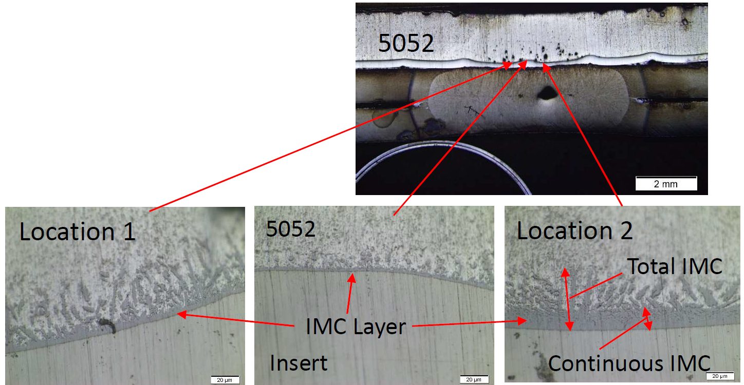
Figure 1: IMC in the Al Alloy 5052 to Stainless-Steel Weld.W-9
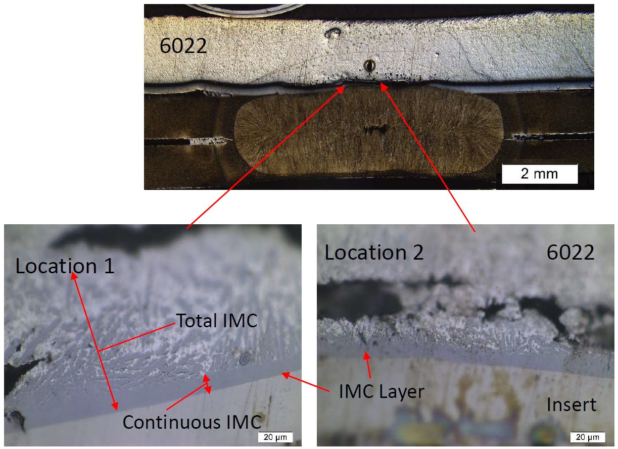
Figure 2: IMC in the Al Alloy 6022 to Stainless-Steel Weld.W-9
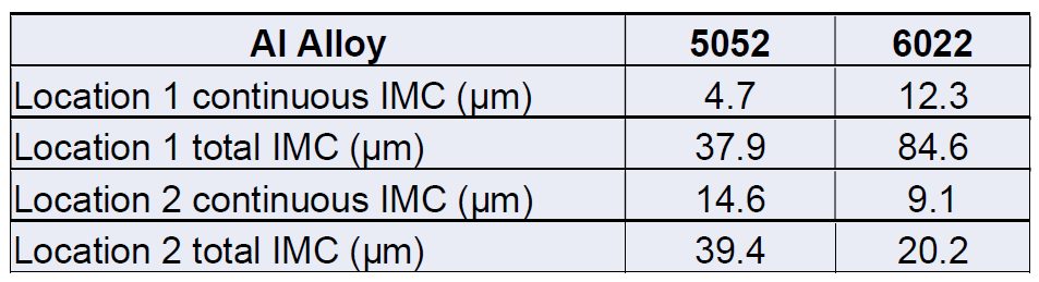
Table 1: IMC Thickness of Both the 5052 Weld and the 6022 Weld.W-9
Referencing Figure 3, the 2T stack-up has a higher tensile strength as well as significantly higher fracture energy absorbed compared to the 3T stack-ups. This is mainly attributed to the failure mode observed in the different stack-ups. The 2T welds had button pullout failure while 3T stack-ups had interfacial Failure.
![Figure 3: Failure Load and Fracture Energy [(A) Al to steel (Al-Us) welds and (B) steel to steel (Us-Us) welds (the 2T 6022 results are from previous work(10))]W-9](https://ahssinsights.org/wp-content/uploads/2021/12/fig4-process.jpg)
Figure 3: Failure Load and Fracture Energy [(A) Al to steel (Al-Us) welds and (B) steel to steel (Us-Us) welds (the 2T 6022 results are from previous work(10))]W-9
The Al 6022 contains higher Si content which likely decreased the growth of the continuous IMC layer but not the overall IMC layer (as seen in Figure 4 and Figure 5) due to higher weld temperatures. The joint strength of the welds in the 3T stack-ups were closer to the expected weld strength unless there was expulsion that caused a 5-kN drop in strength.
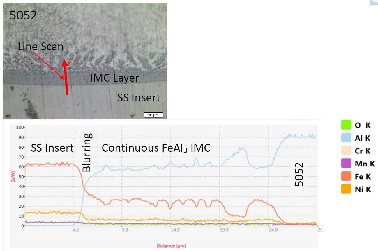
Figure 4: EDS Line Scan of the IMC in Location 2 on the 5052 3T Sample (SS stands for austenitic stainless steel 316).W-9
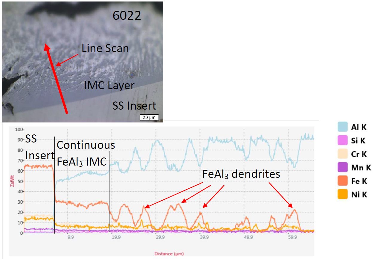
Figure 5: EDS Line Scan of the Intermetallic Layer at Location 1 on the 6022 3T Sample (SS stands for austenitic stainless steel 316).W-9
RSW of Dissimilar Steel
This article is the summary of a paper entitled, “HAZ Softening of RSW of 3T Dissimilar Steel Stack-up”, Y. Lu., et al.L-15
Electromechanical Model
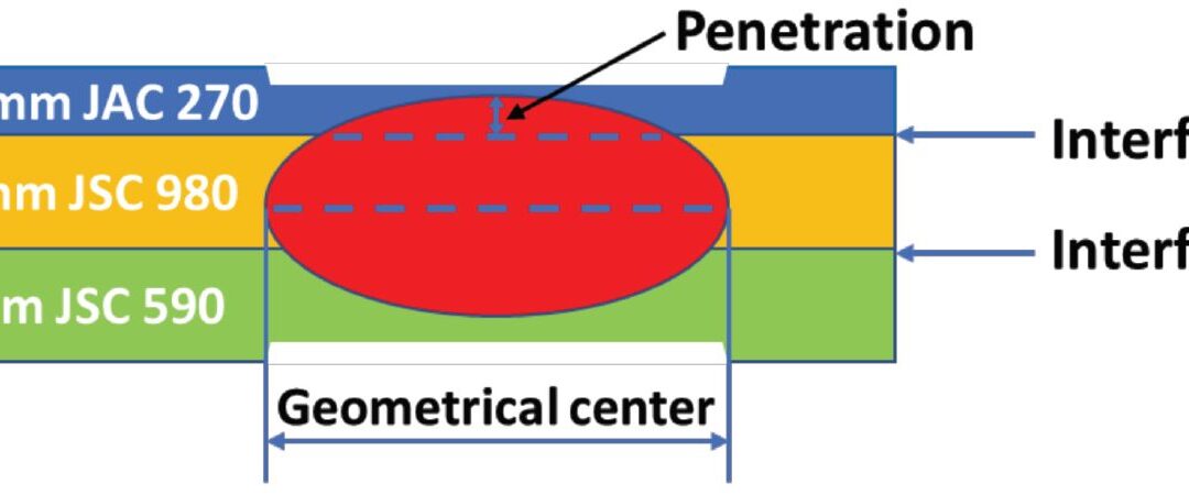
The study discusses the development of a 3D fully coupled thermo-electromechanical model for RSW of a three sheet (3T) stack-up of dissimilar steels. Figure 1 schematically shows the stack-up used in the study. The stack-up chosen is representative of the complex stack-ups used in BIW. Table 1 summarizes the nominal compositions of the three steels labeled in Figure 1.
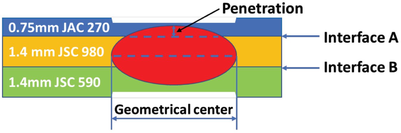
Figure 1: Schematics of the 3T stack-up of 0.75-mm-thick JAC 270/1.4-mm-thick JSC 980/1.4-mm-thick JSC 590 steels.L-15
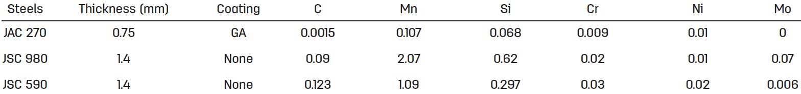
Table 1: Nominal Composition of Steels.L-15
JAC270 is a cold rolled Mild steel with a galvanneal coating having a minimum tensile strength of 270 MPa. JSC590 and JSC980 are bare cold rolled Dual Phase steels with a minimum tensile strength of 590 MPa and 980 MPa, respectively.
The electrodes used were CuZr dome-radius electrodes with a surface diameter of 6 mm. The welding parameters are listed in Table 2.
Table 2: Welding Parameters for Resistance Spot Welding of 3T Stack-Up of Steel Sheets.L-15
Figure 2 shows consistent nugget dimensions between simulation and experiment, supporting the validity of the RSW process model for 3T stack-up. The effect of welding current on nugget penetration into the thin sheet is similar to that on the nugget size. It increases rapidly at low welding current and saturates to 32% when the welding current is higher than 9 kA, as shown in Figure 2C.
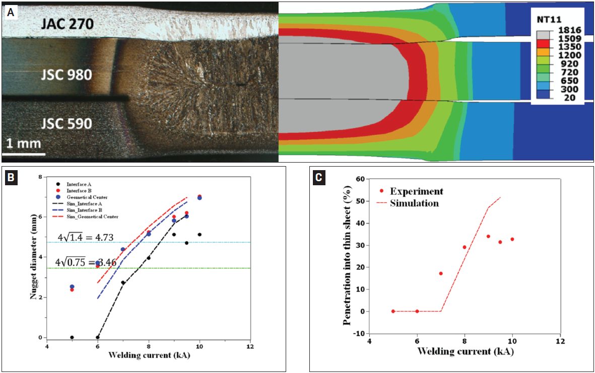
Figure 2: Comparison between experimental and simulated results: A) Nugget geometry at 8 kA; B) nugget diameters; C) nugget penetration into the thin sheet as a function of welding current. In Figure 2A, the simulated nugget geometry is represented by the distribution of peak temperature (in Celsius). The two horizontal lines in Figure 2B represent the minimal nugget diameter at Interfaces A and B calculated, according to AWS D8.1M: 2007, Specification for Automotive Weld Quality Resistance Spot Welding of Steel. Due to limited number of samples available for testing, the variability in nugget dimensions at each welding current was not measuredL-15.
The results for nugget formation during RSW of the 3T stack-up are show in Figures 3-5. Figure 2 shows that, at the start of welding, the contact pressure at interface A (thin/thick) has a higher peak and drops more quickly along the radial direction than that at interface B (thick/thick). Due to the more localized contact area (Figure 3), a high current density can be observed at interface A, as shown in Figure 4A. Additionally, due to the high current density at interface A, localized heating is generated at this interface, as shown in Figure 5A.
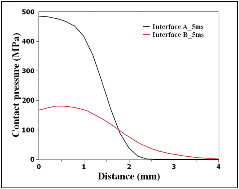
Figure 3: Calculated contact pressure distribution at interfaces A (thin/thick) and B (thick/thick) at a welding time of 5 ms, current of 8 kA, and electrode force of 3.4 L-15
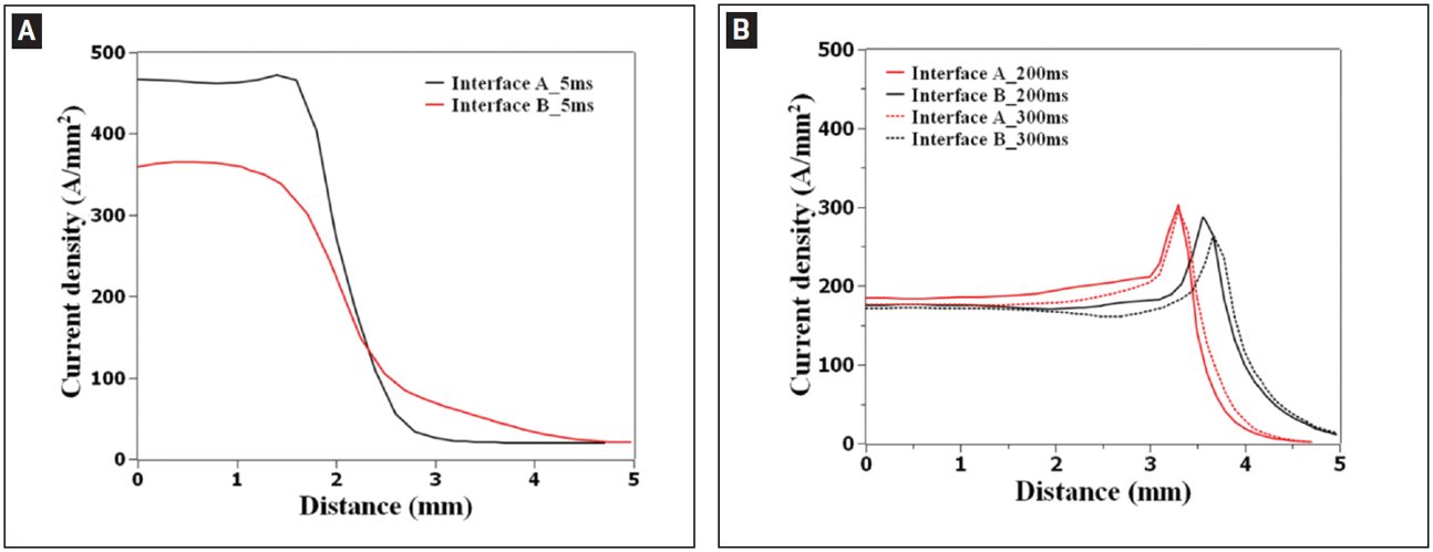
Figure 4: Calculated current density distribution at interfaces A (thin/thick) and B (thick/thick) at welding time of A — 5 ms; B — 200 and 300 ms.L-15
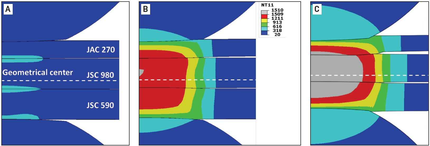
Figure 5: Temperature distribution during resistance spot welding of 3T stack-up at welding times of A) 5 ms; B) 102 ms; C) 300 ms. Welding current is 8 kA and electrode force is 3.4 kN. Calculated temperature is given in Celsius.L-15
As welding time increases, the contact area is expanded, resulting in a decrease of current density. The heat generation rate is shifted from interfaces to the bulk and the peak temperature occurs near the geometrical center of the stack-up.
Figure 6 illustrates that the predicted value corresponds well with the experimental data indicating a sound fitting to the isothermal tempering experimental data.
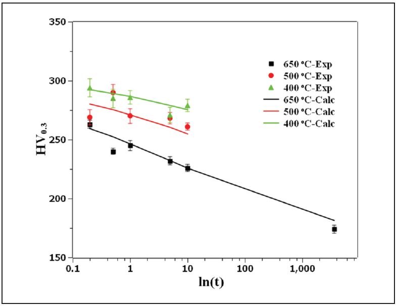
Figure 6: Comparison of the measured hardness with JMAK calculation showing the goodness of fit of the JSC 980 tempering kinetics parameters.L-15
Figure 7 shows the predicted hardness map of RSW 3T stack-up as well as the predicted and measured hardness profiles for JSC 980.
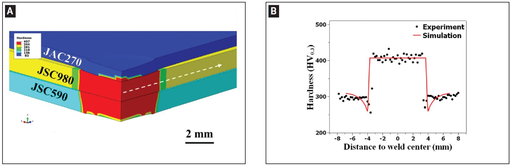
Figure 7: A) Predicted hardness map of resistance spot welded 3T stack-up; B) predicted and measured hardness profiles along the line marked in (A) for JSC 980.L-15
RSW Modelling and Performance
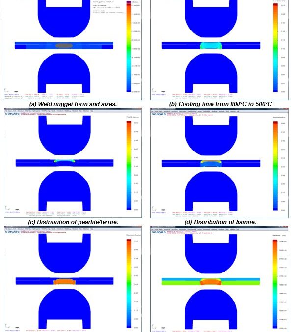
The advantages of numerical simulations for resistance welding are obvious for saving time and reducing costs in product developments and process optimizations. Today’s modeling techniques can predict temperature, microstructure, stress, and hardness distribution in the weld and Heat Affected Zone (HAZ) after welding. Commercial modeling software is available which considers material type, various current modes, machine characteristics, electrode geometry, etc. An example of process simulation results for spot welding of 0.8-mm DC 06 low-carbon steel to 1.2-mm DP 600 steel is shown in Figure 1. Obviously, this technique can apply to dissimilar thicknesses, material types, and geometries. Application of adhesives is also being used with these simulations. This simulation techniques are found to be very beneficial to predict vehicle crashworthiness as it can dramatically reduce the cost of crash evaluations.
You will find several articles in this section describing RSW modelling studies and procedures.
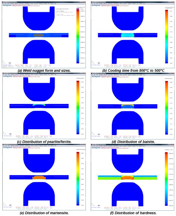
Figure 1: Simulation results with microstructures and hardness distribution for spot welding of 0.8-mm DC06 low-carbon steel to 1.2-mm DP 600 steel.Z-1