The article “Paint Bake Effect on Generation 3 Steel Weld Strength Compared to Other AHSS” by Richard H. Wolf explores the strength increase of resistance spot welds (RSW) in Generation 3 (Gen3) advanced high strength steels (AHSS) due to the paint bake-hardening effect.
These steels, due to their carbon content, may yield welds that can be brittle. A crucial, and often overlooked, aspect of the automotive production process is the paint bake stage, which has been shown to improve the mechanical properties of AHSS welds. In order to correctly assess the strength of a weld, this article proposes to take the paint-bake effect into account.
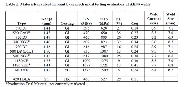
Table 1: Materials tested.
The experimental phase involved various AHSS materials, primarily with 1.5 mm thickness, with differing yield strengths and carbon equivalencies (Ceq). Resistance spot welding was performed under controlled conditions, and the effects of different paint bake temperatures and durations were analyzed.
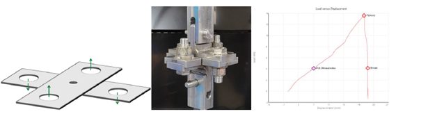
Figure 1: Testing setup
Results indicated that Gen3 steels exhibited a significant increase in weld strength following paint baking, particularly in cross-tension strength (CTS) tests. Higher Ceq values correlated with lower weld strength in the as-welded state, while the paint bake effect tended to equalize these strengths across different alloys.
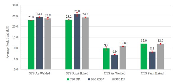
Figure 2: Comparison of shear-tensile strength and cross-tensile strength of different steels with and without paint baking. Especially in cross-tensile testing, a significant increase in load-bearing capacity is visible.
Hardness testing revealed a softening in the heat-affected zone after baking, suggesting that the weld microstructure became more homogenous, which reduces brittleness and improves fracture behavior. The investigation into heterogeneous welding between different steel types further elucidated the contribution of the fusion zone and heat-affected zone to overall weld strength.
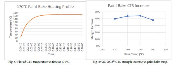
Figure 3: Utilized paint baking profile and cross-tensile strength increase
In conclusion, the paint bake process significantly enhances the strength of AHSS welds, especially for Gen3 steels. This improvement should be factored into weld strength modeling for automotive applications. The author suggests establishing standardized paint bake simulations to ensure weld properties are accurately represented for automotive manufacturers.
Source
Richard H. Wolf, Paint Bake Effect on Generation 3 Steel Weld Strength Compared to Other AHSS
RSW Modelling and Performance
This article summarizes the findings of a paper entitled, “Prediction of Spot Weld Failure in Automotive Steels,”L-48 authored by J. H. Lim and J.W. Ha, POSCO, as presented at the 12th European LS-DYNA Conference, Koblenz, 2019.
To better predict car crashworthiness it is important to have an accurate prediction of spot weld failure. A new approach for prediction of resistance spot weld failure was proposed by POSCO researchers. This model considers the interaction of normal and bending components and calculating the stress by dividing the load by the area of plug fracture.
Background
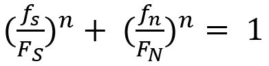
Lee, et al.L-49 developed a model to predict spot welding failure under combined loading conditions using the following equation, based upon experimental results .
|
Equation 1 |
Where FS and FN are shear and normal failure load, respectively, and n is a shape parameter.
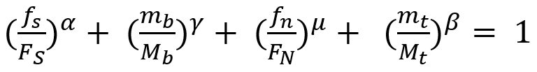
Later, Wung and coworkersW-38 developed a model to predict the failure mode based upon the normal load, shear load, bending and torsion as shown in Equation 2.
 |
Equation 2 |
Here, FS, FN ,Mb and Mt are normal failure load, shear failure load, failure moment and failure torsion of spot weld, respectively. α, β, γ and μ are shape parameters.
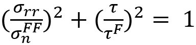
Seeger et al.S-106 proposed a model for failure criterion that describes a 3D polynomial failure surface. Spot weld failure occurs if the sum of the components of the normal, bending and shear stresses are above the surface, as shown in the Figure 1.
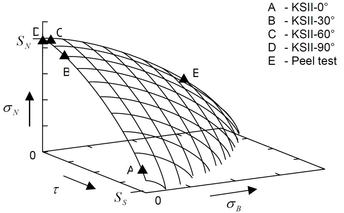
Figure 1: Spot weld failure model proposed by Seeger et al.S-106
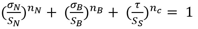
The failure criterion can be expressed via Equation 3.
 |
Equation 3 |
Here, σN , σB , and τ are normal, bending and shear stress of the spot weld, respectively. And nN, nB and nc are the shape parameters. Toyota Motor CorporationL-50 has developed the stress-based failure model as shown in Equation 4.
 |
Equation 4 |
Hybrid Method to Determine Coefficients for Failure Models
This work used a unique hybrid method to determine the failure coefficients for modeling. The hybrid procedure steps are as follows:
- Failure tests are performed with respect to loading conditions.
- Finite element simulations are performed for each experiment.
- Based on the failure loads obtained in each test, the instant of onset of spot weld failure is determined. Failure loads are extracted comparing experiments with simulations.
- Post processing of those simulations gives the failure load components acting on spot welds such as normal, shear and bending loads.
These failure load components are plotted on the plane consisting of normal, shear and bending axes.
The hybrid method described above is shown in Figure 2.L-48
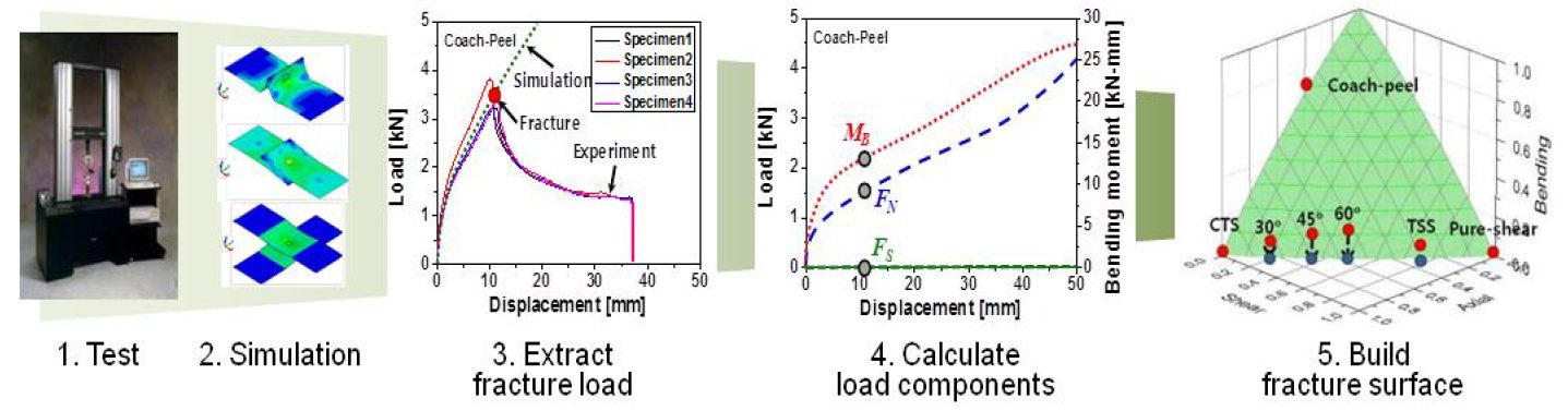
Figure 2: Hybrid method to obtain the failure load with respect to test conditions.L-48
New Spot Weld Failure Model
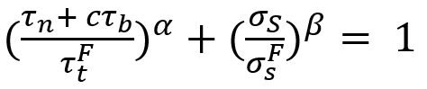
The new proposed spot weld failure model in this paper considers only plug fracture mode as a normal spot weld failure. Secondly normal and bending components considered to be dependent upon each other. Stress generated by normal and bending components is shear, and shear component generates normal stress. Lastly authors have used πdt to calculate the area of stress instead of πd2/4. The final expression is shown in the Equation 5.
 |
Equation 5 |
Here τn is the shear stress by normal load components, σS is the normal stress due to shear load component. And  ,
,  , c, α and β are coefficients.
This work included verification experiments of 42 kinds of homogenous steel stack-ups and 23 heterogeneous stack-ups. The strength levels of the steels used was between 270 MPa and 1500 MPa, and thickness between 0.55 mm and 2.3 mm. These experiments were used to evaluate the model and compare the results to the Wung model.
Conclusions
Overall, this new model considers interaction between normal and bending components as they have the same loading direction and plane. The current developed model was compared with the Wung model described above and has shown better results with a desirable error, especially for asymmetric material and thickness.
Resistance Spot Welding
This article summarizes a paper entitled, “High Strength Steel Spot Weld Strength Improvement through in situ Post Weld Heat Treatment (PWHT)”, by I. Diallo, et al.D-9
The study proposes optimal process parameters and process robustness for any new spot welding configuration. These parameters include minimum quenching time, post weld time, and post-welding current.
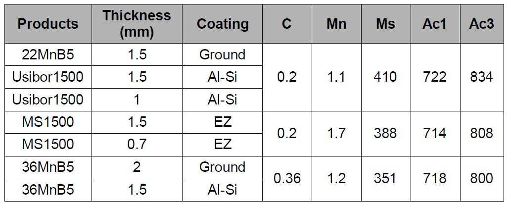
Three different chemical compositions are considered in this study and are listed in Table 1.
Table 1: Chemical composition and metallurgical data of products tested. Formulas used to calculate Ms, Ac1 and Ac3 are from “Andrews Empirical Formulae for the Calculation of Some Transformation Temperatures.”D-9
Welding configurations and process parameters are described in Table 2.
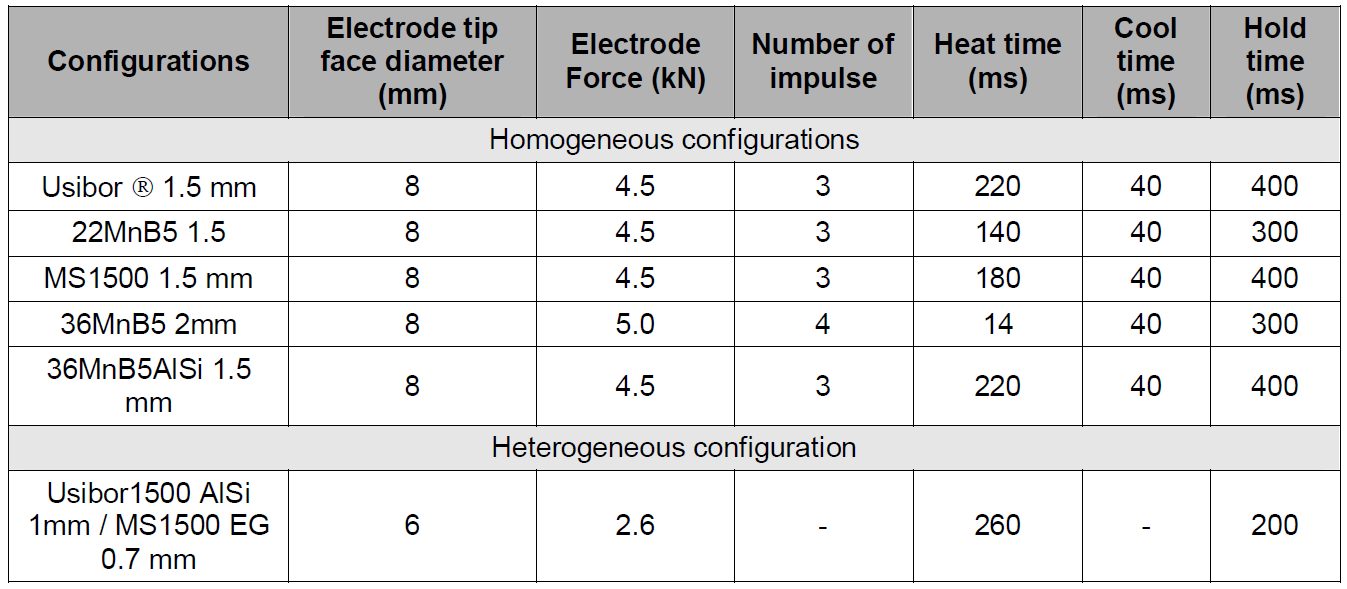
Table 2: Welded configurations and welding parameters used in reference cases.D-9
Cross Tensile Strength for MS1500EG 1.5 mm homogenous configuration is seen in Figure 1. Table 3 lists the reference data for the other configurations in this study.
Figure 1: Cross Tensile Strength for MS1500EG 1.5 mm homogenous configuration as a function of plug (closed symbols) or weld (open symbols) diameter.D-9
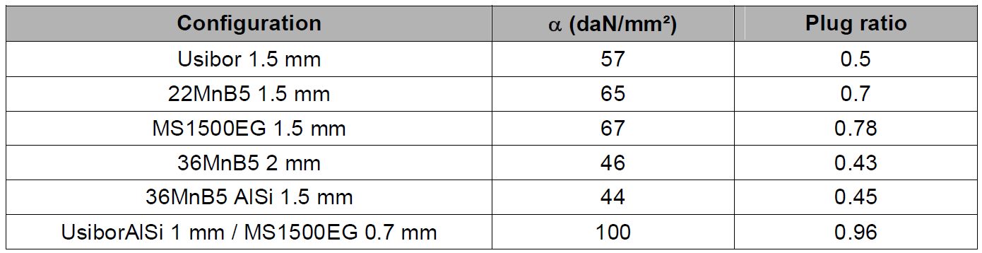
Table 3: Average α and plug ratio along the welding range for reference configurations.D-9
Figure 2 and 3 depict micrographs of welds after PWHT applied on 36MnB5 2 mm homogeneous configuration. These micrographs illustrate the evolution of the microstructure during PWHT and are labeled accordingly. Figure 4 shows the microhardness profiles in the welds described in Figure 3. It is clear that the Mf temperature was reached in the entire weld before application of PWHT.
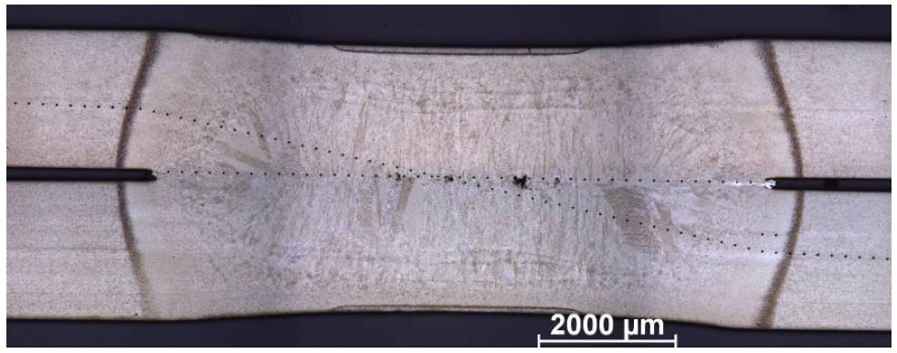
Figure 2: Micrograph of reference weld for 36MnB5 2mm homogeneous configuration.D-9
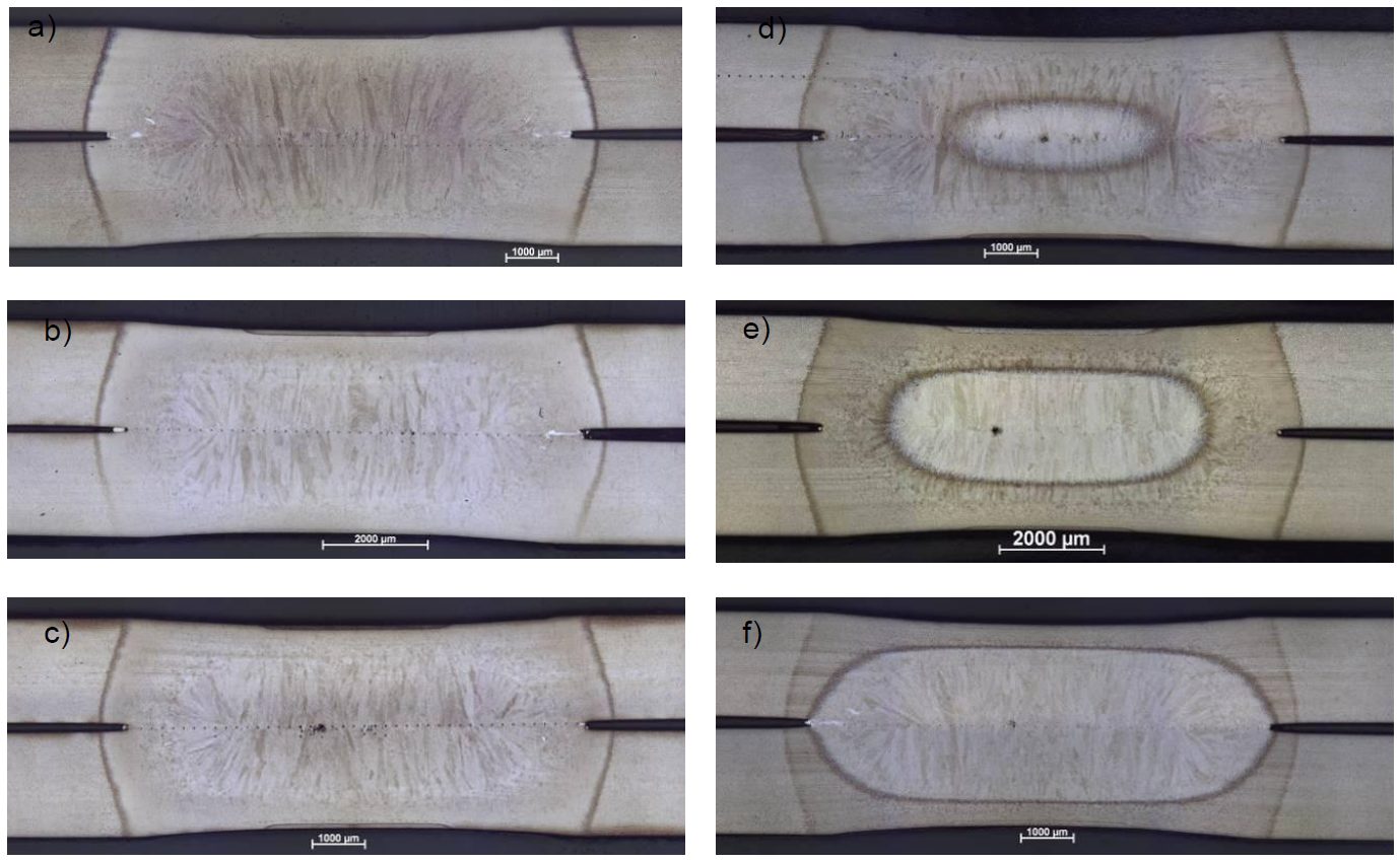
Figure 3: Micrographs of welds after post weld heat treatment applied on 36MnB5 2 mm homogeneous configuration with 70 periods of quenching and post welding current of a) 54%Iw, b) 62%Iw, c) 65% d) 67%Iw, e) 71%Iw and f ) 78%Iw.D-9
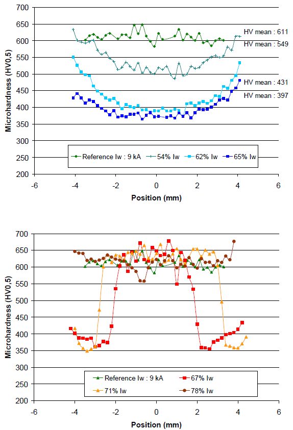
Figure 4: Microhardness profiles in welds after post weld treatment applied on 36MnB5 2mm homogeneous configuration with 70 periods of quenching ; these measurements correspond to micrographs shown in Figure 2 and Figure 3.D-9
Similar methodology was performed on partial quenching examples with AISI coating and electrogalvanized coating. Table 4 lists the minimum quenching times that were determined experimentally for each configuration.
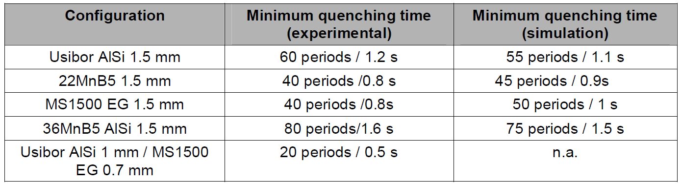
Table 4: Minimum quenching times determined experimentally and through Sorpas simulation.D-9
For selection of post weld time, a slightly different methodology was performed. Optimal quenching time was determined and used to construct the evolution of post weld current range as a function of post weld time as described in Figure 5. This figure shows that post welding current range is stable between 60 and 30 periods of post weld time.
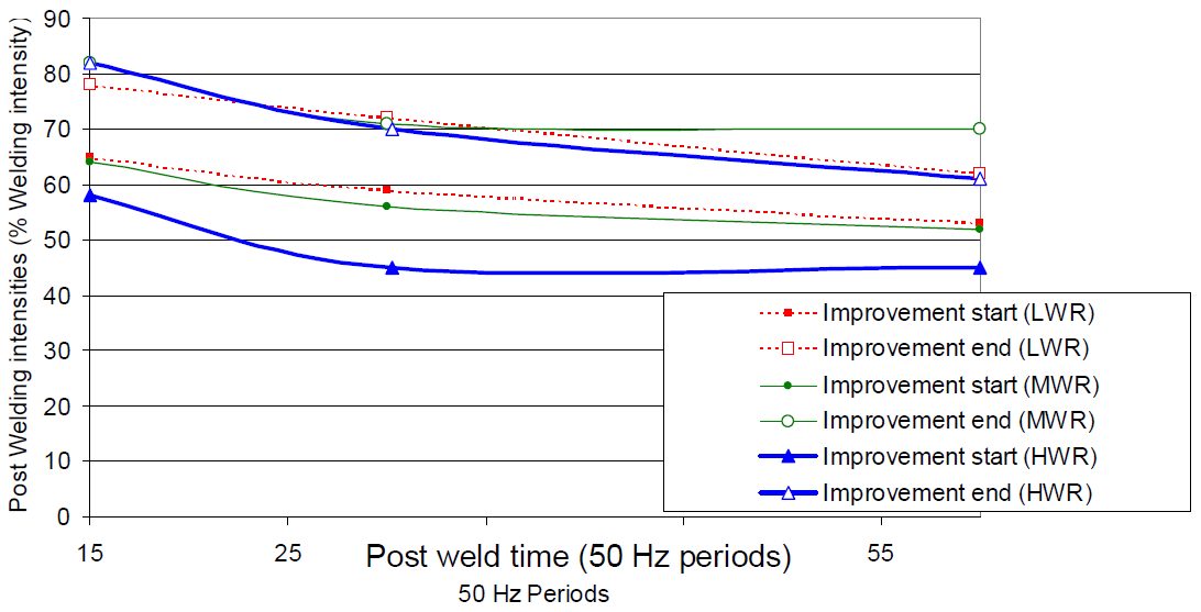
Figure 5: Evolution of post welding current range as a function of post weld time for three welding current levels.D-9
Notch tip hardness measured after different post welding currents has been reported in Figure 6. From this result, a notch tip tempering range is found to be between 400 °C and Ac1.
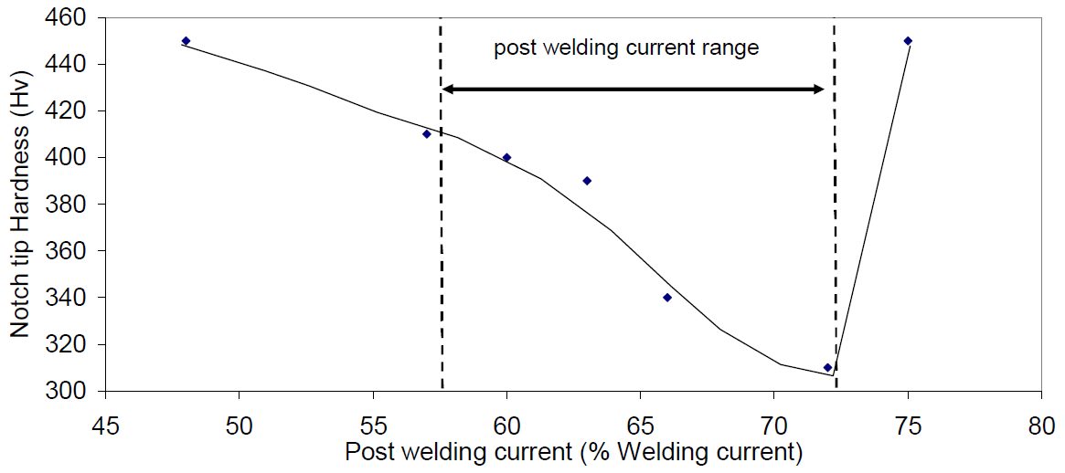
Figure 6: Relationship between measured notch tip hardness and post-welding current (Usibor1500 AlSi 1.5mm, LWR).D-9
Using the notch tip tempering range, a post welding current range can be calculated from Sorpas calculations in Figure 7.
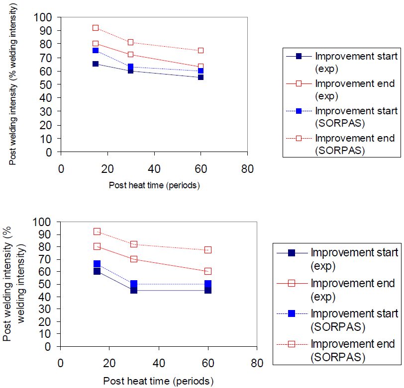
Figure 7: Experimental and numerical post welding current ranges for Usibor1500 AlSi 1.5 mm configuration (above: LWR, below: HWR).D-9
Results are displayed in Figure 8 for post weld time for MS1500 EZ with low welding current LWR.
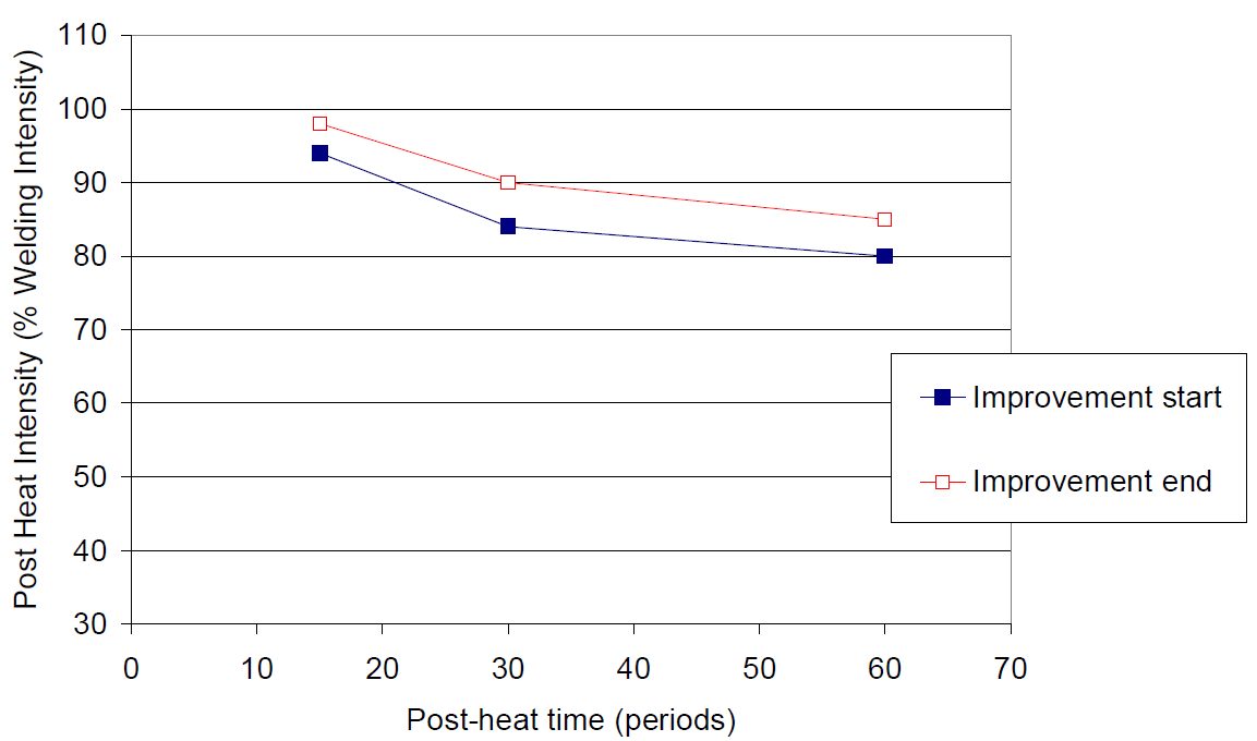
Figure 8: Evolution of post welding current ranges for different post welding times in LWR.D-9
Figure 9 displays results for MS1500 EG 1.5mm configuration.
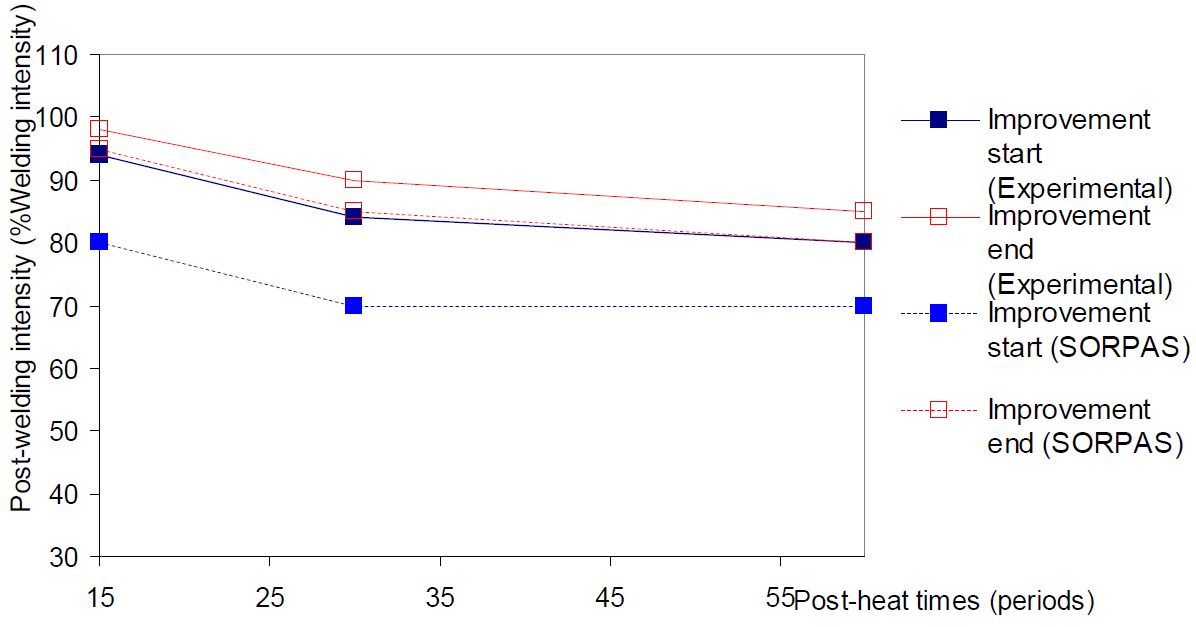
Figure 9: MS1500 EG 1.5 mm configuration experimental and simulated post welding current ranges (LWR).D-9
The same methodology was applied to other configurations and the results are displayed in Table 5.
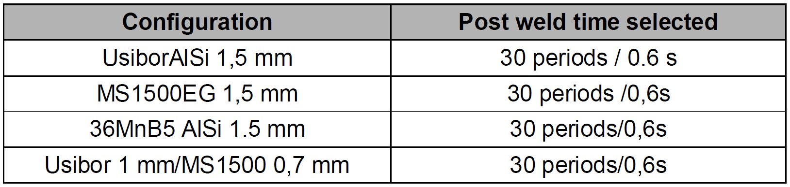
Table 5: Post weld times selected.D-9
Interpolation between experiments was carried out to create a robustness and performance tempering map that is displayed in Figure 10. The map shows tremendous improvement of cross tension strength can be achieved through PWHT. Additionally, the optimal post welding current is around 65% of welding current, and the CTS level reached for LWR and HWR without PWHT is very similar.
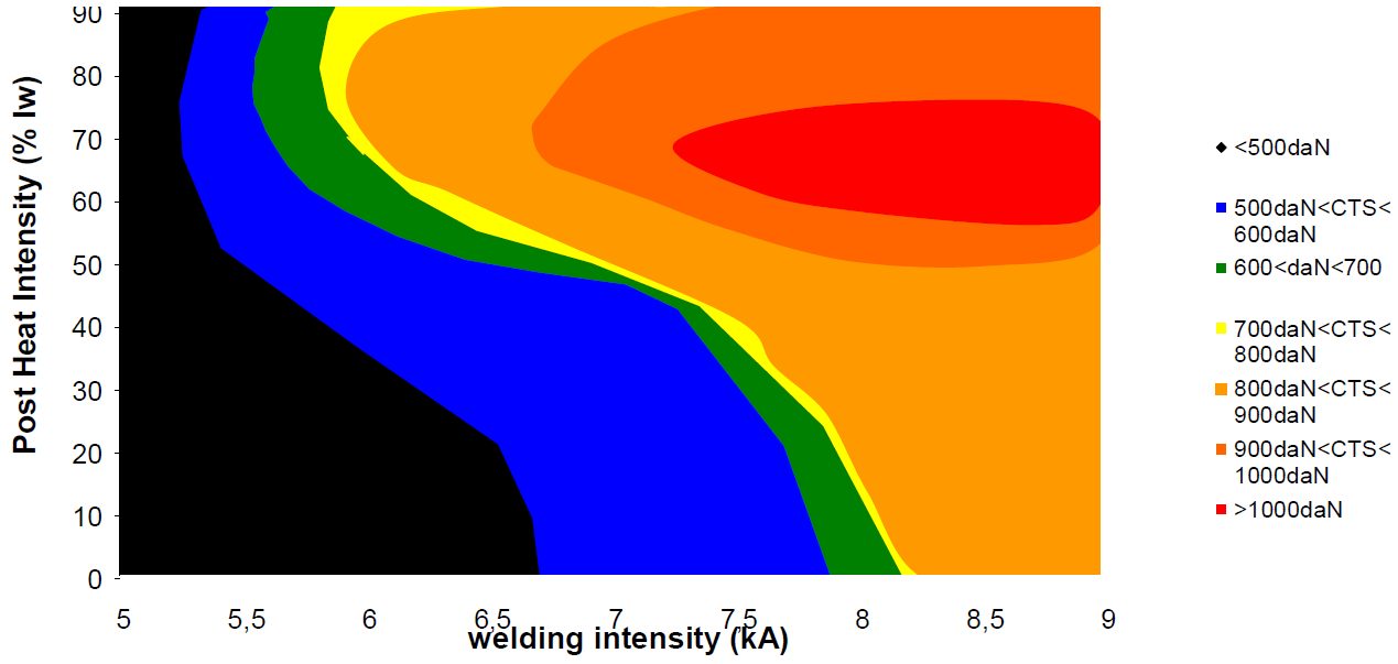
Figure 10: Tempering map for Usibor ® AlSi 1.5 mm homogeneous configuration, drawn after experimental results shown on Figure 9.D-9
Figure 11 displays cross-tension results for Usibor1500 AlSi using the optimized cycle [Metallurgical Post Weld Heat Treatment (MPWHT)].
Figure 11: Comparison of CTS along the welding current range, with and without MPWHT.D-9
Table 6 and Figure 12 display all the reference and MPWHT spot weld performance after Cross-Tension testing.
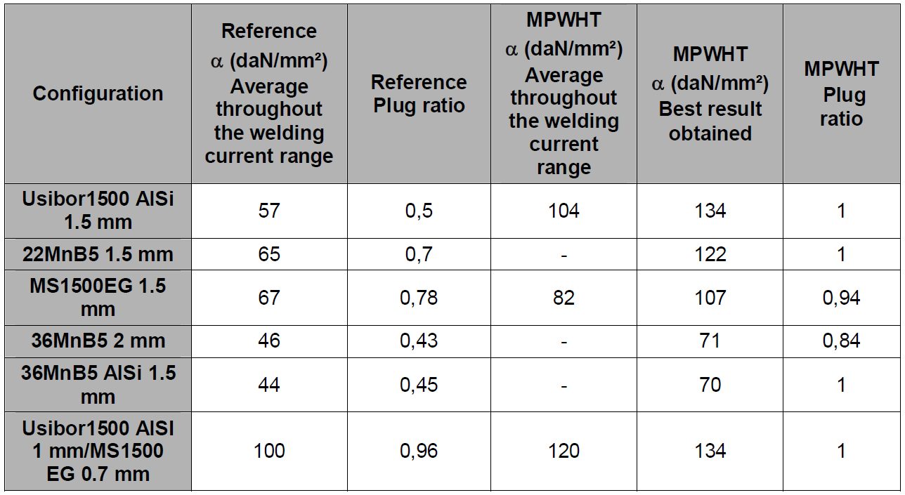
Table 6: ɑ coefficients and plug ratios for reference and with post treatment for all the configurations.D-9
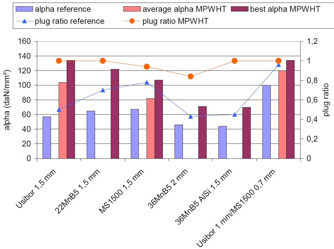
Figure 12: ɑ coefficients and plug ratios for reference and with post treatment for all the configurations.D-9
MPWHT, aiming at tempering the martensite formed during spot welding of Advanced High-Strength Steels, has been studied for several configurations both experimentally and numerically. The methodology proposed in this study is available to determine the optimal process parameters and the process robustness for any new configuration. Among the major results brought by this study:
- A minimum quenching time is necessary to fully transform the weld into martensite before post weld heat treatment; this time can be determined based on metallographic observations, and depends strongly on sheets thickness, chemistry and coating.
- The post weld time is not very sensitive to the configuration welded; 0.6 s seems a reasonable time, although it may be reduced further.
- The post welding current can be simply expressed as a percentage of the welding current, the efficient level being then constant along the welding current range.
- A range of post welding currents can be determined, allowing an efficiency of the post weld heat treatment process. Tempering maps allow common visualization of the welding current and post welding current ranges in two dimensions, to characterize the whole process robustness.
- MPWHT is very efficient in improving the mechanical weld performance in opening mode; cross-tension strength can be doubled in some cases; the process efficiency depends on the chemistry of the grades.
- In case of heterogeneous configuration, the so-called “positive deviation” can give a good performance to the weld even without MPWHT, limiting the improvement brought after post treatment.
Automotive Welding Process Comparison
Introduction
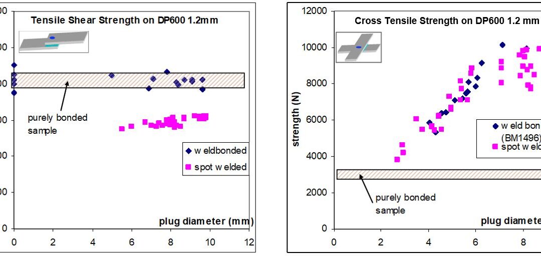
A solution to improve the spot weld strength is to add a HS adhesive to the weld. Figure 1 illustrates the strength improvement obtained in static conditions when crash adhesive (example: Betamate 1496 Dow Automotive) is added. The trials are performed with 45-mm-wide and 16-mm adhesive bead samples.
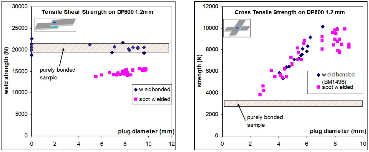
Figure 1: TSS and CTS on DP 600.A-16
Another approach to improve the strength of welds is done by using laser welding instead of spot welding. The technologies based on remote welding optics have been introduced and a high productivity can be obtained. The effective welding time is maximized and a wide variety of weld geometries becomes feasible. Compared to spot welding, the main advantage of laser welding, regarding mechanical properties of the joint, is the possibility to adjust the weld dimension to the requirement. One may assume that, in tensile shear conditions, the weld strength depends linearly of the weld length (Figure 2).
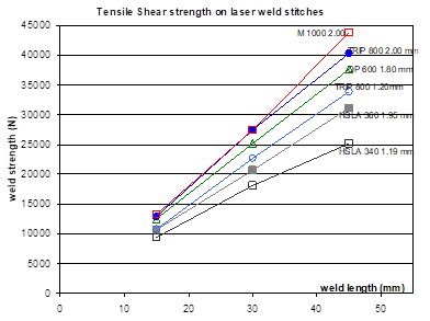
Figure 2: Tensile-shear strength on laser weld stitches of different length.A-16
Comparing spot weld strength with laser weld strength cannot be restricted to the basic tensile shear test. Tests were performed to evaluate the weld strength in both quasi-static and dynamic conditions under different solicitations, on various UHSS combinations. The trials were performed on a high-speed testing machine, at 5 mm/min for the quasi-static tests and 0.5 m/s for the dynamic tests (pure shear, pure tear or mixed solicitation) (Figure 3). The strength at failure and the energy absorbed during the trial have been measured. It should be noticed that the energy absorbed depends also on the deformation of the sample. However, as all the trials were made according to the same sample geometry, the comparison of the results is relevant. Laser stitches were done with a 27-mm length. C- and S-shape welds were performed with the same overall weld length. This lead s to various apparent length and width of the welds. A shape factor, expressed as the ratio width/length of the weld, can be defined according to Table 1.
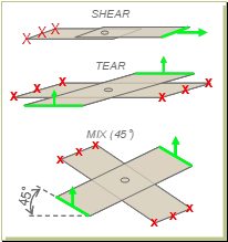
Figure 3: Sample geometry for quasi-static and dynamic tests. A-16
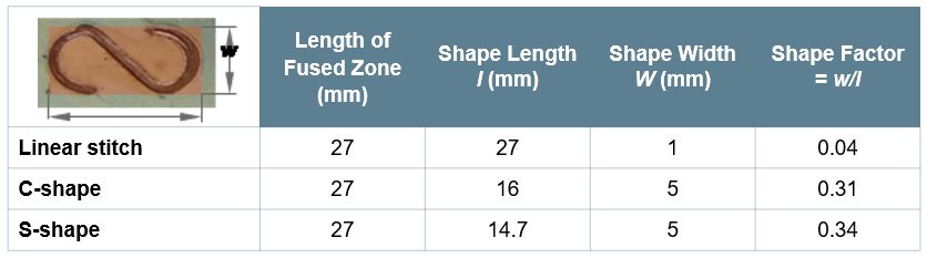
Table 1: Shape factor definition.A-16
The weld strength at failure can be easily described with an elliptic representation, with major axes representing pure shear and normal solicitation (Figure 4). For a reference spot weld corresponding to the upper limit of the weldability range, globally similar weld properties can be obtained with 27-mm laser welds. The spot weld equivalent length of 25-30 mm has been confirmed on other test cases on UHSS in the 1.5- to 2-mm range thickness. It has also been noticed that the spot weld equivalent length is shorter on thin mild steel (approximately 15-20 mm). This must be considered in case of shifting from spot to laser welding on a given structure. There is no major strain rate influence on the weld strength; the same order of magnitude is obtained in quasi-static and dynamic conditions.
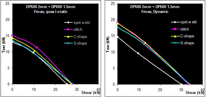
Figure 4: Quasi-static and dynamic strength of welds, DP 600 2 mm+1.5 mm.A-16
The results in terms of energy absorbed by the sample are seen in Figure 5. In tearing conditions, both the strength at fracture and energy are lower for the spot weld than for the various laser welding procedures. In shear conditions, the strength at fracture is equivalent for all the welding processes. However, the energy absorption is more favorable to spot welds. This is due to the different fracture modes of the welds. IF fracture is observed on the laser welds under shearing solicitation (Figure 6). Even if the strength at failure is as high as for the spot weds, this brutal failure mode leads to lower total energy absorption.
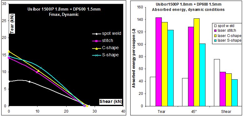
Figure 5: Strength at fracture and energy absorption of HF1500P 1.8-mm + DP 600 1.5-mm samples for various welding conditions. A-16
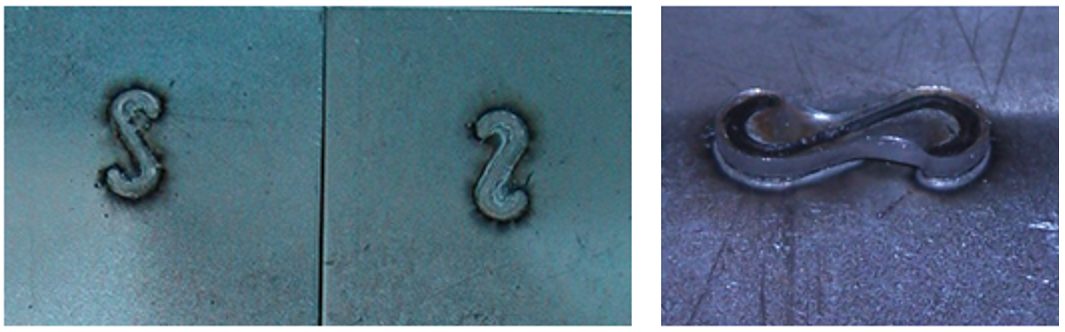
Figure 6: IF fracture mode (left), “plug-out” fracture mode (right).A-16
Figure 7 represents the energy absorbed by omega-shaped structures and the corresponding number of welds that fail during the frontal crash test (here on TRIP 800 grade). It appears clearly that laser stitches have the highest rate of fracture during the crash test (33%). In standard spot welding, some weld fractures also occur. It is known that UHSS are more prone to partial IF fracture on coupons, and some welds fail as well during the crash test. By using either Weld-Bonding or adapted laser welding shape, there is no more weld fractures during the test, even if the parts are severely crashed and deformed. As a consequence, higher energy absorption is also observed.
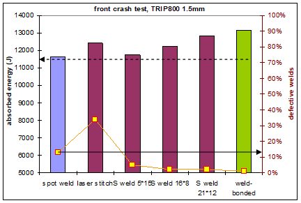
Figure 7: Welding process and weld shape influence on the energy absorption and weld integrity on frontal crash tests. A-16
Regarding stiffness, up to 20% improvement can be obtained. The best results are obtained with continuous joints, and particularly using adhesives. Adhesive bonding and weld- bonding lead to the same results of the stiffness improvement only being due to the adhesive, not to the additional welds.
Figure 8 shows the evolution of the torsional stiffness with the joining process.
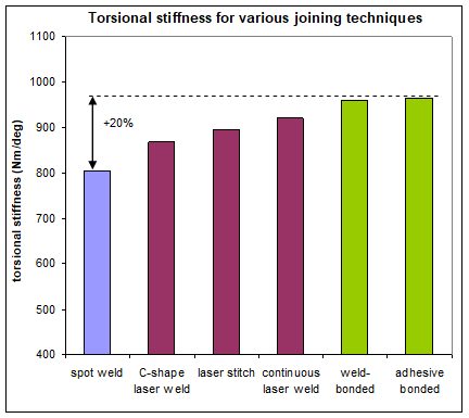
Figure 8: Evolution of the torsional stiffness with the joining process.A-16
Optimized laser joining design leads to same performances as a weld bonded sample regarding fracture modes seen in Figure 9.
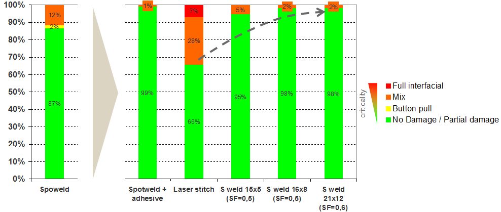
Figure 9: Validation test case 1.2-mmTRIP 800/1.2-mm hat-shaped TRIP 800.
Top-hat crash boxes were tested across a range of AHSS materials including DP 1000. The spot weld’s energy absorbed increased linearly with increasing material strength. The adhesives were not suitable for crash applications as the adhesive peels open along the entire length of the joint. The welded bond samples perform much better than conventional spot welds. Across the entire range of materials there was a 20-30% increase in mean force when WB was used. The implications of such a large increase in crash performance are very significant. The results show that when a 600 MPa steel is weld bonded it can achieve the same crash performance as a 1000 MPa steel in spot-welded condition. It is also possible that some down gauging of materials could be achieved, but as the strength of the crash structure is highly dependent upon sheet thickness only small gage reductions would be possible.
Figure 10 shows the crash results for spot-welded and weld-bonded AHSS.
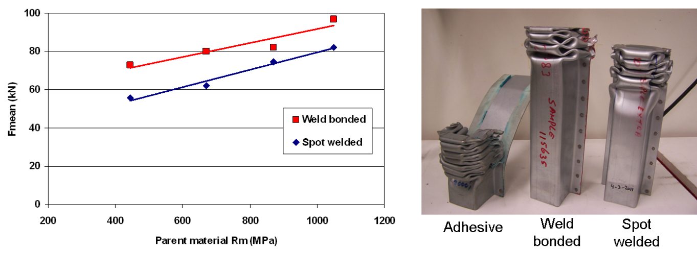
Figure 10: Crash results for spot-welded and weld-bonded AHSS.
There are numerous welding processes available for the welding of AHSS in automotive applications. Each of these processes has advantages and disadvantages that make them more or less applicable for particular applications. These qualities include joint efficiency, joint fit-up and design, joint strength, and stiffness, fracture mode, and cost effectiveness (equipment cost, production rates, etc.). The following data can allow for comparisons to be made for automotive application welding and joining processes, as well as possible repair substitutions.
Many tests were performed using lap and coach joints, reduced specimen overlap distance, and adjusted weld sizes to more closely represent typical joints consistent with automotive industry acceptance criteria. The tests were aimed at providing a baseline reference for a wide variety of welding and joining processes and material combinations. In general, there was no correlation between joint efficiency, normalized energy, and normalized stiffness. Joint efficiency was calculated by dividing the peak load of the joint by the peak load of the parent metal. Some processes, joint configurations and material combinations have high joint efficiency and energy, while others result in high joint efficiency but low energy. Few processes showed high values for all metrics across all materials and joint configurations (Figure 11). It was observed that peak loads tended to increase, on average, as material strength increased for lap joints (Figure 12). However, joint efficiency generally decreased as material strength increased. Therefore, joint strength did not increase in proportion to parent material strength increase for most of the processes and materials studied. Coach joints generally showed lower joint efficiency and stiffness than lap joints (Figure 13). Process and material combinations should be selected based on the required performance, joint design, and cost.A-12
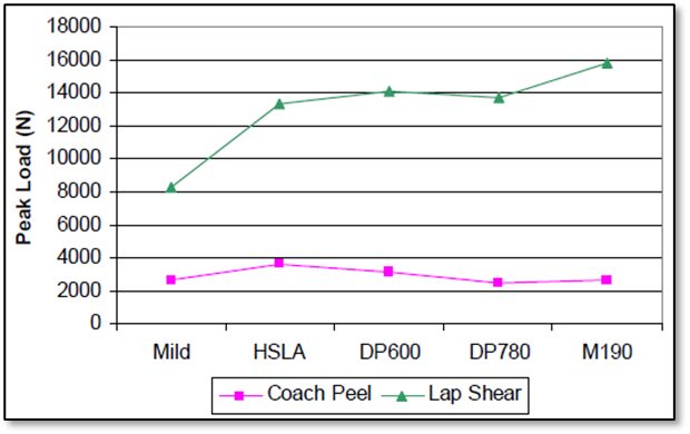
Figure 11: Average peak loads (all processes combined).A-12
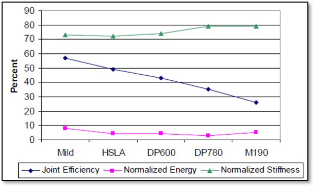
Figure 12: Lap shear average joint efficiency, normalized energy and stiffness (all processes combined).A-12
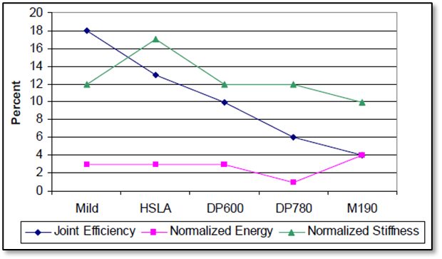
Figure 13: Coach peel average joint efficiency, normalized energy and stiffness (all processes combined).A-12
All Processes General Comparison
Numerous tests were performed using the most popular automotive joining processes including RSW, GMAW/brazing, laser welding/brazing, mechanical fasteners, and adhesive bonding. Joint efficiency and normalized energy of all the processes were compared for HSLA steels, DP 600 samples, DP 780 samples, and M190 samples. Joint efficiency was calculated as the peak load of the joint divided by the peak load of the parent metal. Energy was calculated as the area under the load/displacement curve up to peak load.
The materials used consisted of 1.2-mm EG HSLA, 1.2-mm galvanized DP 600, 1.0-mm GA DP 780, and 1.0-mm EG M190. The testing configuration matrix (Table 2) lists the materials and process combinations studied. The tolerance of weld lengths is ±10%. Lap-shear joints were centered in the overlap for all processes except lap fillet welds and brazes. Coach-peel joints were centered in the overlap for all processes (Figure 14). A-12
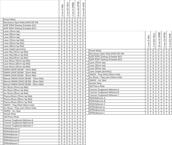
Table 2: Lap-shear (left) and coach-peel (right) test configuration matrix.A-12
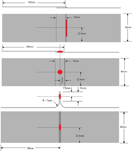
Figure 14: Lap-shear and coach-peel set-up.A-12
DP 600 samples, DP 780 samples, and M190 samples. Joint efficiency was calculated as the peak load of the joint divided by the peak load of the parent metal. Energy was calculated as the area under the load/displacement curve up to peak load.
Self-piercing riveting with adhesive gave the greatest overall joint efficiency for the HSLA lap shear tests, while laser obtained the largest normalized energy (Figure 15a and 15b).
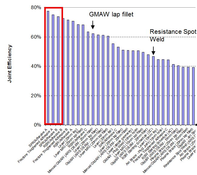
Figure 15a: Joint efficiency of HSLA lap-shear tests for all processes.A-12
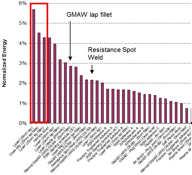
Figure 15b: Normalized energy of HSLA lap-shear tests for all processes.A-12
Self-penetrating riveting with adhesive gave the greatest overall values for both joint efficiency and normalized energy for lap shear testing of DP 600 samples (Figure 16a and 16b). However, coach peel testing of DP 600 obtained the best results with laser welding (Figure 17).
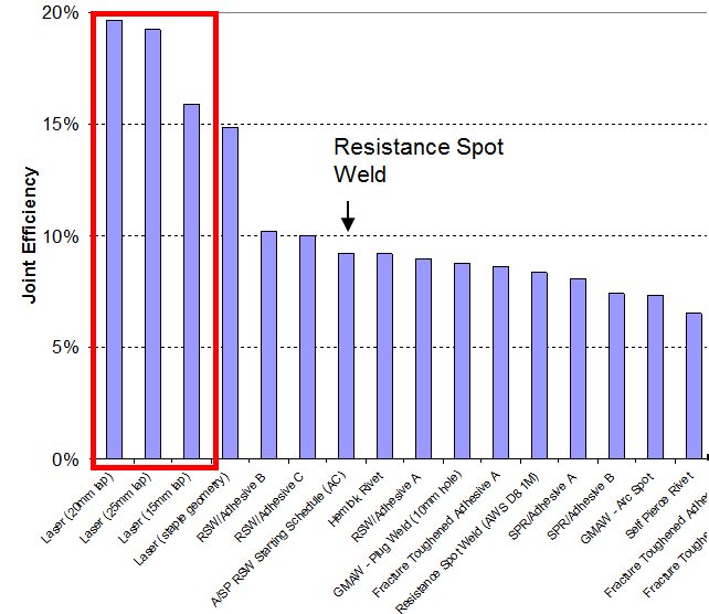
Figure 17a: Joint efficiency of DP 600 lap shear for all processes.A-12
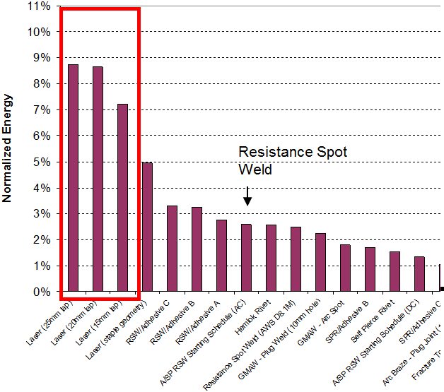
Figure 16b: Normalized energy of DP 600 lap shear for all processes.A-12
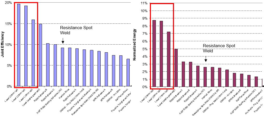
Figure 17: Joint efficiency and normalized energy of DP 600 coach peel for all processes.A-12
For the DP 780 lap-shear test, the best results out of all the tested processes were from laser/MIG welding, leading in both joint efficiency and normalized energy (Figure 18). Full laser welding produced the best results for coach-peel tests of the DP 780 samples (Figure 19).
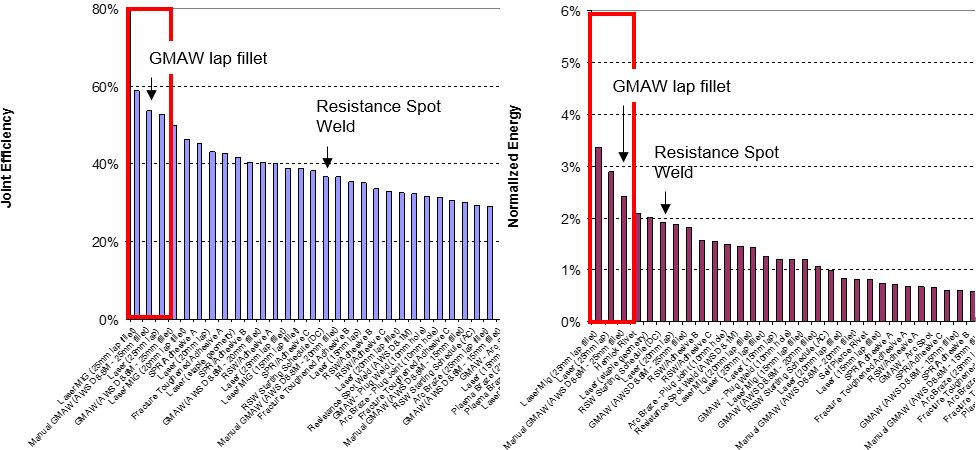
Figure 18: Joint efficiency and normalized energy of DP 780 lap shear for all processes.A-12
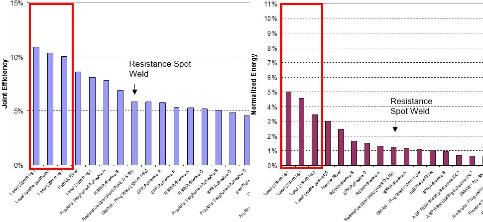
Figure 19: Joint efficiency and normalized energy of DP 780 coach peel for all processes.A-12
The M190 lap-shear samples had the best joint efficiency using RSW with adhesive, but full laser welding gave better normalized energy (Figure 20). The coach peel tests also had the best normalized energy with full laser welding. The best joint efficiency of the coach peel tests was produced from laser welding with staples (Figure 21).
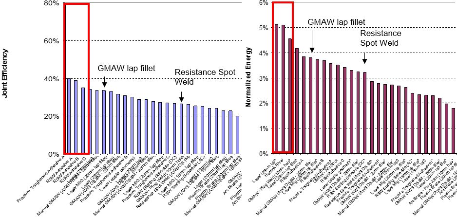
Figure 20: Joint efficiency and normalized energy of M190 lap shear for all processes.A-12
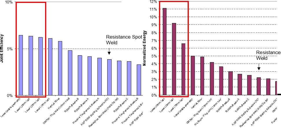
Figure 21: Joint efficiency and normalized energy of M190 coach peel for all processes.A-12
Cost Effectiveness Comparison: Spot Welding to Spot/Laser Welding Mixture
When automotive manufacturers are weighing the advantages and disadvantages of RSW to those of a spot/laser welding mixture process, cost effectiveness is a major concern. Spot/laser mixture welding has 38% lower operation cost compared to full spot welding because the laser installation performs more welds than a spot welding robot. Also, there are fewer robots to maintain and less consumables. The global cost is similar, but the spot/laser solution is about 4% less expensive overall. Figure 22 shows a cost comparison of spot welding and spot/laser welding.
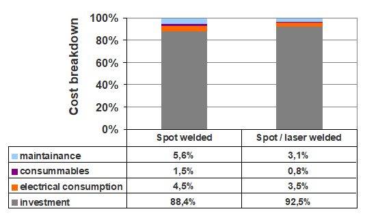
Figure 22: Cost comparison of spot welding and spot/laser welding.A-16
GMAW Compared to Laser Welding
When comparing the advantages and disadvantages of GMAW to those of laser welding in automotive applications, joint efficiency is a key subject. Numerous welds were made using both processes on 15- and 25-mm-thick pieces of materials varying in strength. All results showed that laser welding continuously had greater joint efficiency than GMAW (Figure 23).
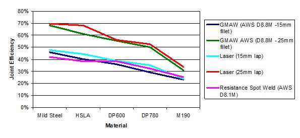
Figure 23: Joint efficiency of GMAW and laser welding for various steel strengths.
Back To Top