Testing and Characterization
Many demands are placed on automotive body structures which influence the material selection process. The impact on safety, manufacturability, and longevity are among the most critical, with each of these balanced against cost and environmental concerns.
Formed sheet metal products experience a complex series of deforming, cutting, and joining before being placed in a body structure, where these components will be subjected to complex loading conditions during the product life cycle. Understanding the failure limits and the conditions which produce failure allows for the design of body structures which can withstand these demands.
Testing helps determine whether a metal is suitable for its intended use. Different tests characterize specific performance aspects. Historically, manufacturers relied on tensile testing to understand metal flow. However, new tests help us understand the behavior of new steel grades and their interactions more thoroughly with new manufacturing technologies.
Mechanical Properties
R-Value, The Plastic Anisotropy Ratio
The r-value, which is also called the Lankford coefficient or the plastic strain ratio, is the ratio of the true width strain to the true thickness strain at a particular value of length strain, indicated in Equation 1. Strains of 15% to 20% are commonly used for determining the r-value of low carbon sheet steel. Like n-value, the ratio will change depending on the chosen reference strain value.
Equation 1
The normal anisotropy ratio (rm) defines the ability of the metal to deform in the thickness direction relative to deformation in the plane of the sheet. rm, also called r-bar (i.e. r average) is the “normal anisotropy parameter” in the formula for Equation 2:
Equation 2
where r0, r90, and r45 are the r-value determined in 0, 90, and 45 degrees relative to the rolling direction.
For rm values greater than one, the sheet metal resists thinning. Values greater than one improve cup drawing (Figure 1), hole expansion, and other forming modes where metal thinning is detrimental. When For rm values are less than one, thinning becomes the preferential metal flow direction, increasing the risk of failure in drawing operations.

Figure 1: Higher r-value is associated with improved deep drawability.
High-strength steels with tensile strength greater than 450 MPa and hot-rolled steels have rm values close to one. Therefore, conventional HSLA and Advanced High-Strength Steels (AHSS) at similar yield strengths perform equally in forming modes influenced by the rm value. However, r-value for higher strength grades of AHSS (800 MPa or higher) can be lower than one and any performance influenced by r-value would be not as good as HSLA of similar strength. For example, AHSS grades may struggle to form part geometries that require a deep draw, including corners where the steel is under circumferential compression on the binder. This is one of the reasons why higher strength level AHSS grades should have part designs and draw dies developed as “open ended”.
A related parameter is Delta r (∆r), the “planar anisotropy parameter” in the formula shown in Equation 3:
Equation 3
Delta r is an indicator of the ability of a material to demonstrate a non-earing behavior. A value of 0 is ideal in can making or the deep drawing of cylinders, as this indicates equal metal flow in all directions, eliminating the need to trim ears prior to subsequent processing.
Testing procedures for determining r-value are covered in Citations A-44, I-15, J-14.
![N-Value]()
Mechanical Properties
N-Value, The Strain Hardening Exponent
Metals get stronger with deformation through a process known as strain hardening or work hardening, resulting in the characteristic parabolic shape of a stress-strain curve between the yield strength at the start of plastic deformation and the tensile strength.
Work hardening has both advantages and disadvantages. The additional work hardening in areas of greater deformation reduces the formation of localized strain gradients, shown in Figure 1.

Figure 1: Higher n-value reduces strain gradients, allowing for more complex stampings. Lower n-value concentrates strains, leading to early failure.
Consider a die design where deformation increased in one zone relative to the remainder of the stamping. Without work hardening, this deformation zone would become thinner as the metal stretches to create more surface area. This thinning increases the local surface stress to cause more thinning until the metal reaches its forming limit. With work hardening the reverse occurs. The metal becomes stronger in the higher deformation zone and reduces the tendency for localized thinning. The surface deformation becomes more uniformly distributed.
Although the yield strength, tensile strength, yield/tensile ratio and percent elongation are helpful when assessing sheet metal formability, for most steels it is the n-value along with steel thickness that determines the position of the forming limit curve (FLC) on the forming limit diagram (FLD). The n-value, therefore, is the mechanical property that one should always analyze when global formability concerns exist. That is also why the n-value is one of the key material related inputs used in virtual forming simulations.
Work hardening of sheet steels is commonly determined through the Holloman power law equation:
 Equation 1
where
σ is the true flow stress (the strength at the current level of strain),
K is a constant known as the Strength Coefficient, defined as the true strength at a true strain of 1,
ε is the applied strain in true strain units, and
n is the work hardening exponent
Rearranging this equation with some knowledge of advanced algebra shows that n-value is mathematically defined as the slope of the logarithmic true stress – true strain curve. This calculated slope – and therefore the n-value – is affected by the strain range over which it is calculated. Typically, the selected range starts at 10% elongation at the lower end to the lesser of uniform elongation or 20% elongation as the upper end. This approach works well when n-value does not change with deformation, which is the case with mild steels and conventional high strength steels.
Conversely, many Advanced High-Strength Steel (AHSS) grades have n-values that change as a function of applied strain. For example, Figure 2 compares the instantaneous n-value of DP 350/600 and TRIP 350/600 against a conventional HSLA350/450 grade. The DP steel has a higher n-value at lower strain levels, then drops to a range similar to the conventional HSLA grade after about 7% to 8% strain. The actual strain gradient on parts produced from these two steels will be different due to this initial higher work hardening rate of the dual phase steel: higher n-value minimizes strain localization.

Figure 2: Instantaneous n-values versus strain for DP 350/600, TRIP 350/600 and HSLA 350/450 steels.K-1
As a result of this unique characteristic of certain AHSS grades with respect to n-value, many steel specifications for these grades have two n-value requirements: the conventional minimum n-value determined from 10% strain to the end of uniform elongation, and a second requirement of greater n-value determined using a 4% to 6% strain range.
Plots of n-value against strain define instantaneous n-values, and are helpful in characterizing the stretchability of these newer steels. Work hardening also plays an important role in determining the amount of total stretchability as measured by various deformation limits like Forming Limit Curves.
Higher n-value at lower strains is a characteristic of Dual Phase (DP) steels and TRIP steels. DP steels exhibit the greatest initial work hardening rate at strains below 8%. Whereas DP steels perform well under global formability conditions, TRIP steels offer additional advantages derived from a unique, multiphase microstructure that also adds retained austenite and bainite to the DP microstructure. During deformation, the retained austenite is transformed into martensite which increases strength through the TRIP effect. This transformation continues with additional deformation as long as there is sufficient retained austenite, allowing TRIP steel to maintain very high n-value of 0.23 to 0.25 throughout the entire deformation process (Figure 2). This characteristic allows for the forming of more complex geometries, potentially at reduced thickness achieving mass reduction. After the part is formed, additional retained austenite remaining in the microstructure can subsequently transform into martensite in the event of a crash, making TRIP steels a good candidate for parts in crush zones on a vehicle.
Necking failure is related to global formability limitations, where the n-value plays an important role in the amount of allowable deformation at failure. Mild steels and conventional higher strength steels, such as HSLA grades, have an n-value which stays relatively constant with deformation. The n-value is strongly related to the yield strength of the conventional steels (Figure 3).

Figure 3: Experimental relationship between n-value and engineering yield stress for a wide range of mild and conventional HSS types and grades.K-2
N-value influences two specific modes of stretch forming:
- Increasing n-value suppresses the highly localized deformation found in strain gradients (Figure 1).
A stress concentration created by character lines, embossments, or other small features can trigger a strain gradient. Usually formed in the plane strain mode, the major (peak) strain can climb rapidly as the thickness of the steel within the gradient becomes thinner. This peak strain can increase more rapidly than the general deformation in the stamping, causing failure early in the press stroke. Prior to failure, the gradient has increased sensitivity to variations in process inputs. The change in peak strains causes variations in elastic stresses, which can cause dimensional variations in the stamping. The corresponding thinning at the gradient site can reduce corrosion life, fatigue life, crash management and stiffness. As the gradient begins to form, low n-value metal within the gradient undergoes less work hardening, accelerating the peak strain growth within the gradient – leading to early failure. In contrast, higher n-values create greater work hardening, thereby keeping the peak strain low and well below the forming limits. This allows the stamping to reach completion.
- The n-value determines the allowable biaxial stretch within the stamping as defined by the forming limit curve (FLC).
The traditional n-value measurements over the strain range of 10% – 20% would show no difference between the DP 350/600 and HSLA 350/450 steels in Figure 2. The approximately constant n-value plateau extending beyond the 10% strain range provides the terminal or high strain n-value of approximately 0.17. This terminal n-value is a significant input in determining the maximum allowable strain in stretching as defined by the forming limit curve. Experimental FLC curves (Figure 4) for the two steels show this overlap.

Figure 4: Experimentally determined Forming Limit Curves for mils steel, HSLA 350/450, and DP 350/600, each with a thickness of 1.2mm.K-1
Whereas the terminal n-value for DP 350/600 and HSLA 350/450 are both around 0.17, the terminal n-value for TRIP 350/600 is approximately 0.23 – which is comparable to values for deep drawing steels (DDS). This is not to say that TRIP steels and DDS grades necessarily have similar Forming Limit Curves. The terminal n-value of TRIP grades depends strongly on the different chemistries and processing routes used by different steelmakers. In addition, the terminal n-value is a function of the strain history of the stamping that influences the transformation of retained austenite to martensite. Since different locations in a stamping follow different strain paths with varying amounts of deformation, the terminal n-value for TRIP steel could vary with both part design and location within the part. The modified microstructures of the AHSS allow different property relationships to tailor each steel type and grade to specific application needs.
Methods to calculate n-value are described in Citations A-43, I-14, J-13.
![N-Value]()
Mechanical Properties
Total Elongation to Fracture
Deformation continues in the local neck until fracture occurs. The amount of additional strain that can be accommodated in the necked region depends on the microstructure. Inclusions, particles, and grain boundary cracking can accelerate early fracture. Total elongation is measured from start of deformation to start of fracture. Two extensometer gauge lengths are commonly used: A50 (50mm or 2 inches) and A80 (80 mm).
In the past, limited automation and measurement equipment necessitated the use of a non-repeatable technique defined in ASTM E8A-24 and ISO 6892-1I-7 as “elongation after fracture.” Here, the operator attempts to position the two fractured strips back together and hand measures the distance between two gauge marks on the sample.
Tensile testing combined with data acquisition systems are much more commonplace today. According to ASTM E8, the elongation at fracture shall be taken as the strain measured just prior to when the force falls below 10 % of the maximum force encountered during the test. Both elastic strains and plastic strains are included in the measurement.

Figure 1 : Total elongation is measured from start of deformation to start of fracture.
![N-Value]()
Mechanical Properties
Forming forces need to exceed the yield strength for plastic deformation to occur and an engineered stamping to be produced. If a metal structure is loaded to a level below the yield strength, only elastic deformation occurs, and the load can be removed. With no permanent (plastic) deformation, the metal returns to its original shape.
On the stress-strain curve, yielding occurs where the initial linear region transitions to the non-linear portion. This transition does not occur always at a clearly visible well-defined point. Consistent yield strength measurement is facilitated by defining how this parameter should be determined. Two techniques are used when working with sheet metals. The most common method is to draw a line parallel to the modulus line at an offset strain of 0.2%. The intersection stress becomes what is defined at the “0.2% offset yield strength” (Figure 1). This value is referred to as Rp0.2. The second technique is drawing a vertical line at the 0.5% strain value until it crosses the stress-strain curve. This determines the “yield strength at 0.5% extension under load,” abbreviated as Rt0.5 (Figure 2). These techniques result in similar – but not identical – values for yield strength.

Figure 1: 0.2% offset yield strength, determined by offset of a line parallel to the modulus line by 0.2% strain.

Figure 2: Yield strength at 0.5% extension under load, determined by a vertical line offset from the origin by 0.5% strain
Some metals have yield point elongation (YPE) or Lüders bands. Deforming metal is locked in place by interstitial carbon and nitrogen atoms and other restrictive features of the microstructure. Load increases with little corresponding deformation – or put another way, stress increases with only an incremental increase in strain. The highest stress reached is known as the upper yield strength or upper yield point. Once a band of deformed (yielded) metal breaks free from being pinned by dislocations in the microstructure, the stress drops and there is an increase in strain. The lowest stress reached is known as the lower yield strength or lower yield point (Figure 3). The bands of deforming metal are known as Lüders bands, named after one of the people first observing the phenomenon. Lüders deformation continues at approximately a constant stress until the entire sample has yielded, and the sample begins to work harden. The total strain associated with this type of deformation is known as yield point elongation, or YPE. Stabilized, interstitial-free, vacuum degassed steel, such as ULC EDDS are not at risk of aging, and will not exhibit YPE. For those grades susceptible to YPE, leveling prior to sheet forming will minimize this tendency.

Figure 3: Defining upper yield stress, lower yield stress, and yield point elongation.
Since springback is proportional to the yield strength of the steel, knowing the yield strength allows some estimation of relative springback. Figure 4 compares mild steel, HSLA 700Y/800T, and MS 1500 AHSS having a 1400MPa yield strength. The relative magnitude of springback is indicated by the arrows shown on the horizontal axis, and reflects the increase of springback with yield strength.
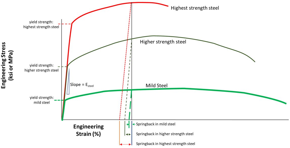
Figure 4: Springback is proportional to yield strength.