G-13
Citation:
G-13. R. Geyer, UCSB Automotive Energy & GHG Model, Mar 14, 2017.

G-13. R. Geyer, UCSB Automotive Energy & GHG Model, Mar 14, 2017.
This article summarizes a paper entitled, “RSW of 22MnB5 at Overlaps with Gaps-Effects, Causes, and Countermeasures”, by J. Kaars, et al.K-12
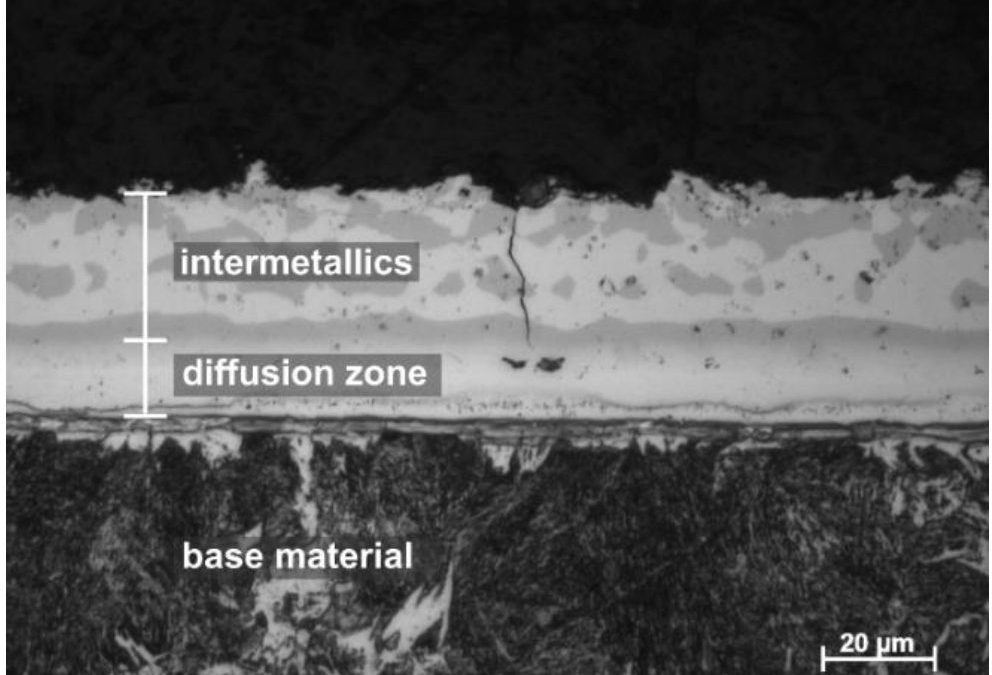
This study aims to elaborate on the influencing mechanisms of gaps on the welding result. Welding experiments at artificial gaps and finite element analysis (FEA) of the welding process have been used to investigate the matter. In both methods, the same configuration of two 1.5-mm-thick 22MnB5+AS150 welded with electrodes of the type ISO 5821 B0-16-20-40-6-30 was considered. Tensile tests yielded an ultimate tensile strength (UTS) of the press-hardened material of 1481 ± 53 MPa with a strain to fracture of 7.5 ± 0.26%. A microsection of the coating morphology after heat treatment can be found in Figure 1.
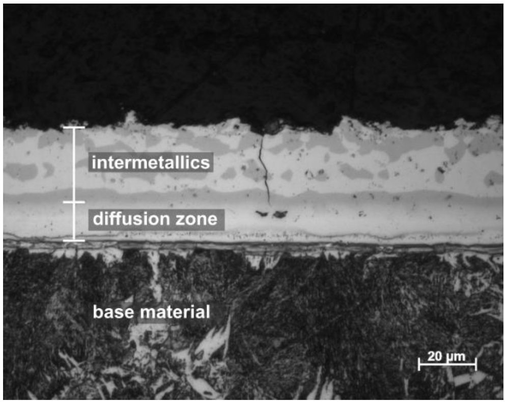
Figure 1: Morphology of the Aluminum-Silicon Coating.K-12
To set up an artificial and reproducible gap between the sheets, a dedicated fixture was used. It is displayed in Figure 2. All welding experiments were carried out with a 6-kN electrode force.
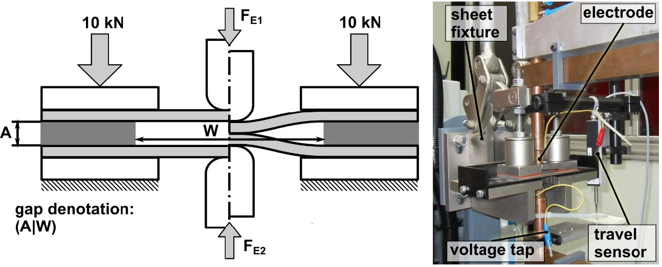
Figure 2: Fixture for Welding at Artificial Gaps, Definition of Quantities.K-12
In Table 1, the parameter variations of the gaps investigated in this work are presented.

Table 1: List of Gap Parameters Investigated.K-12
A 7-kN maximum denting force was observed at the gap (10|60). With a gap of (10|40) the gap could not be closed with the machines’ 8-kN clamping force capacity. In comparative tests on mild steel for deep drawing a clamping force of about 2 kN was required to overcome the gap (10|60) (see Figure 3). The main effects diagram of the denting force clearly shows that the average denting force gets smaller with increasing support width and becomes larger with increasing gap clearance.
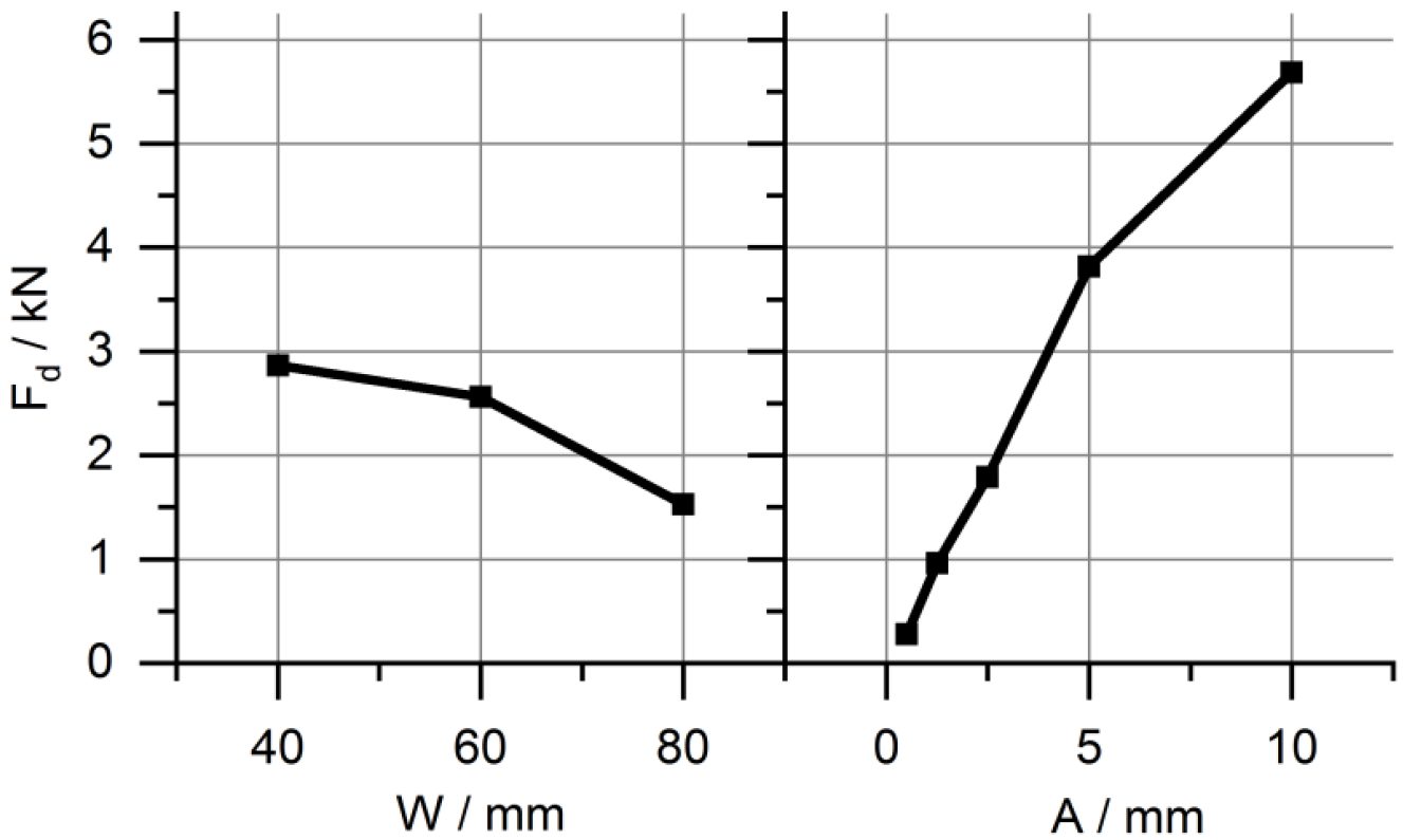
Figure 3: Main Effects Diagram of the Denting Force.K-12
In Figure 4, the achieved nugget diameters at different gaps using a constant machine setting of Iw,f = 6.4 kA are displayed.
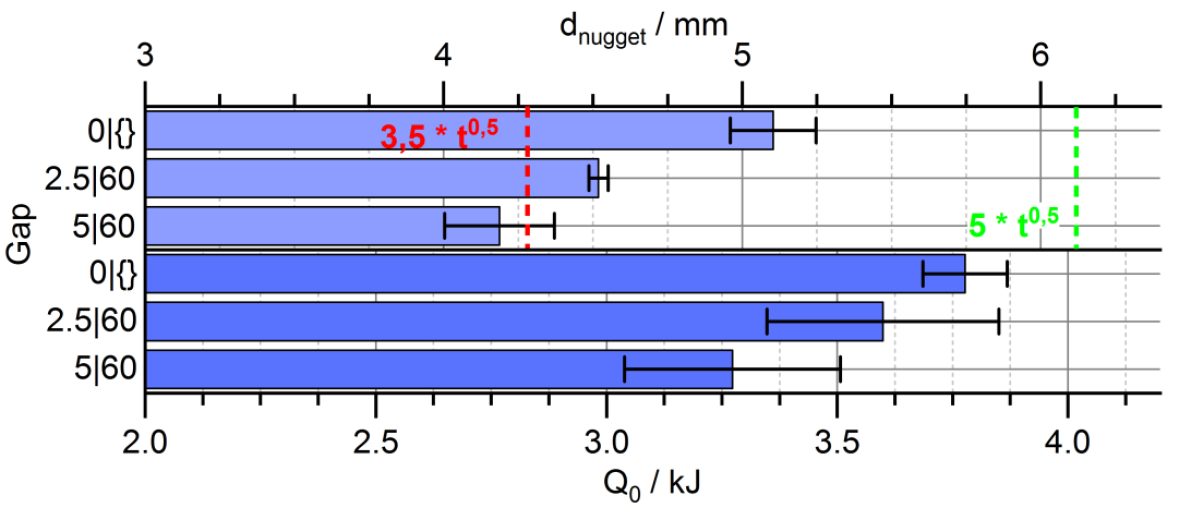
Figure 4: Effect of Gaps on Nugget Diameter, Absolute and Relative Results.K-12
A two-staged welding program, starting with a preheat current followed by a larger finishing current proved to yield the best welding results with the material used, cf., Figure 5. In Figure 5, the applied welding current program along with the measured and computed total resistance curve is displayed.
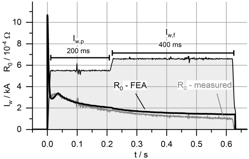
Figure 5: Exemplary Total Resistance Curve of a Weld without Gap, Measured and Computed Results.K-12
The FEA model can represent the welding process in terms of nugget diameter, dynamic resistance curve, and total electric energy with great accuracy. In Figure 6, the partial resistances of the weld as computed by FEA are composed.
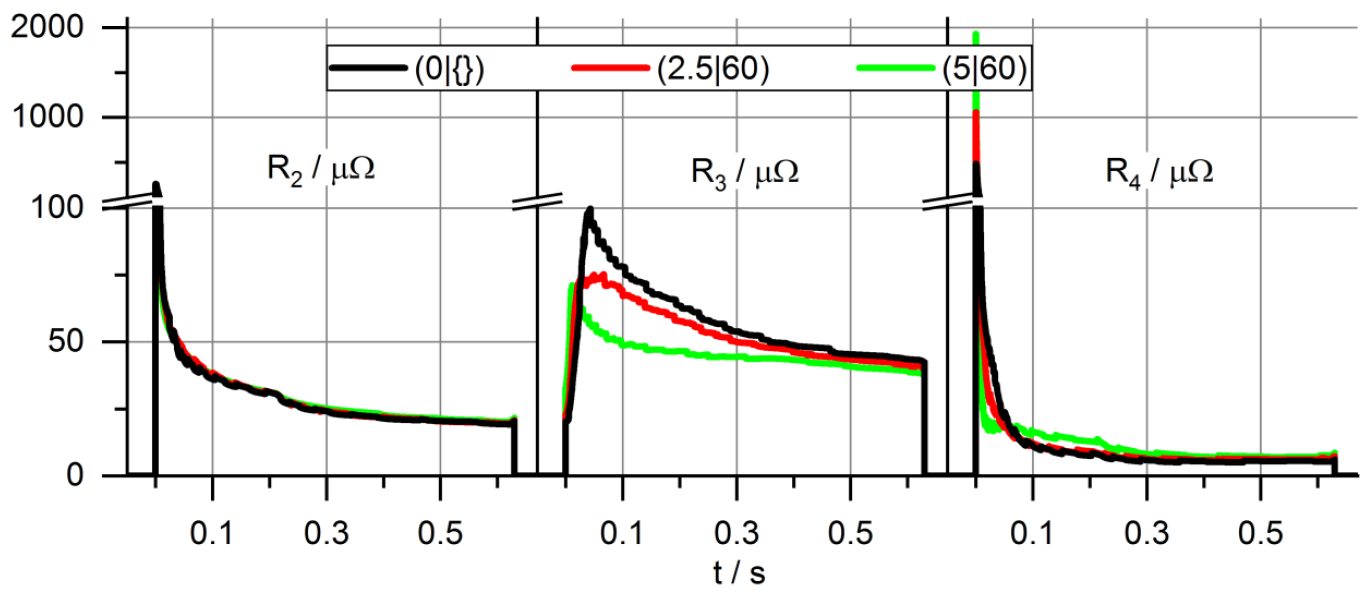
Figure 6: Partial Electrical Resistances at Different Gap Configurations.K-12
In the top section of Figure 7, the computed sheet thickness curve during the process for different gaps is presented. Increased electrode indentation during welding at gaps is the reason for reduced resistance and, therefore, results in reduced nugget diameters. The lower section of Figure 7 shows the plastic strains in the sheets along with a visibly reduced sheet thickness.
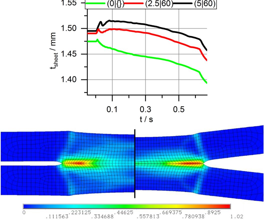
Figure 7: Dynamic Sheet Thickness (up) and Plastic Strain in millimeters at Different Gaps (low, to scale).K-12
Additional welding experiments were performed to clarify, if increased welding current can counter the gap effect and maintain the energy level of the weld. The results are shown in Figure 8. They prove that increased weld current is sufficient to not only maintain the nugget diameter at gaps, but moreover increase it.
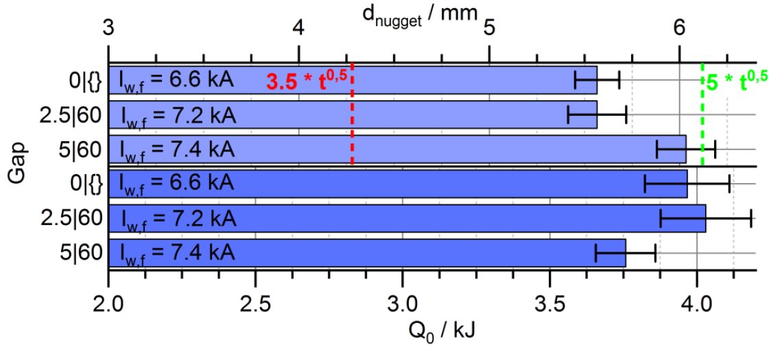
Figure 8: Nugget Diameter and Energy of Spot Welds near the Splash Limit at Overlaps with Gap.K-12
Results of further investigations on the weldability lobe of the joint are composed in Figure 9.. It is visible that with increasing gap the current range shifts toward larger currents and gets narrower.
This article summarizes a paper by W. Mohr and N. Kapustka, EWI, entitled, “Fatigue of GMAW-P Lap Joints in Advanced High-Strength Steels.”M-13
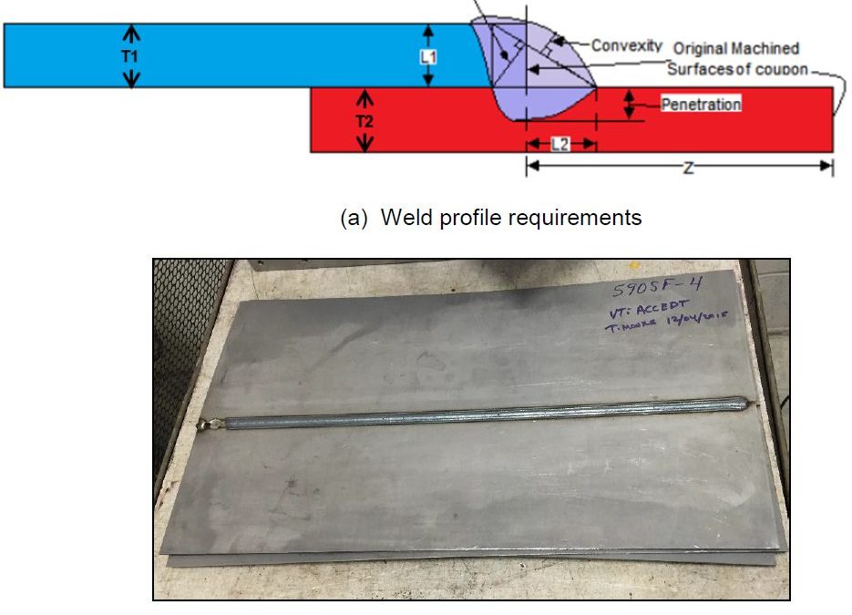
EWI has performed fatigue tests on welds from four Advanced High-Strength Steels (AHSS) in the uncoated condition. The materials were provided in three thicknesses as follows, 2.0-mm DP 780, 1.8-mm 590 SF, 2.0-mm DP 980, and 2.8-mm CP 800. Referring to Figure 1(a), welding parameters were selected to meet the weld profile requirements listed below:
The travel speed to achieve such combinations was 23 mm/s for three of the sheets and 13 mm/s for the 2.8-mm-thick CP 800. Figure 1 shows a completed panel.
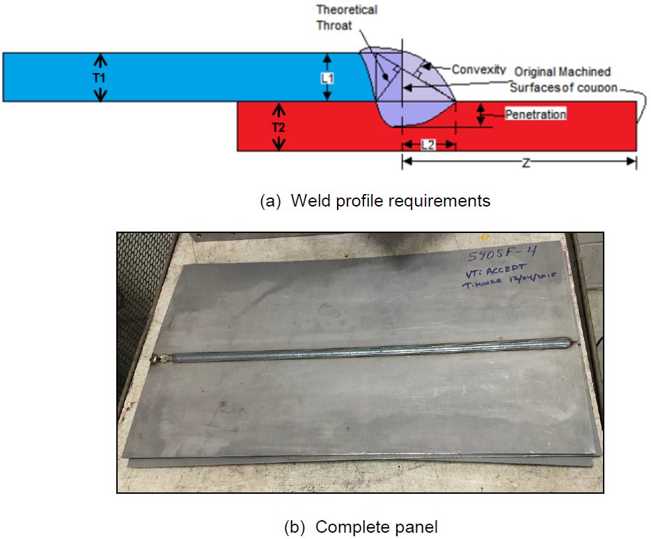
Figure 1: Completed Panel.M-13
Specimens were cut from the lap-welded panels in a configuration recommended by Z 2275, with minimum reduced sections of 20-mm wide, with 20-mm radii on both sides to a full width of 30 mm, as shown in Figure 2.
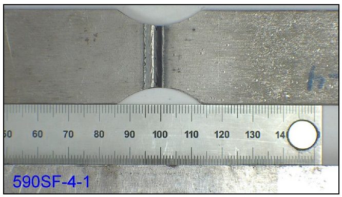
Figure 2: Specimen Design.M-13
Fixtures for the bend testing had eight, 6.3-mm radius rollers, four on top and four on the bottom, with offsets of the roller centers to accommodate the lap-joint configuration and the differing sheet thicknesses. The interior span was 120 mm, while the exterior span was 210 mm. The full bending fixture, with a specimen inserted, is shown in Figure 3.
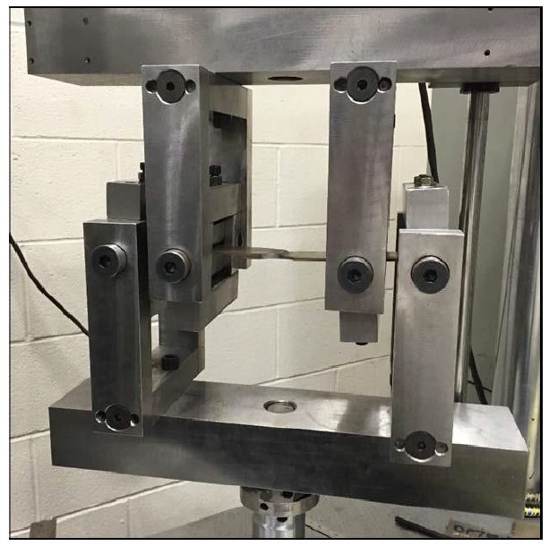
Figure 3: Bending Test Fixture.M-13
Weld profiles were achieved that met the weld profile requirements for each sheet material type. These weld profiles are shown for the four sheet materials in Figure 4. Fatigue testing results in tension at R = 0.3 gave lifetimes between 30,000 and 9 million cycles, with run-outs at 10 million cycles, as shown in Figure 5.
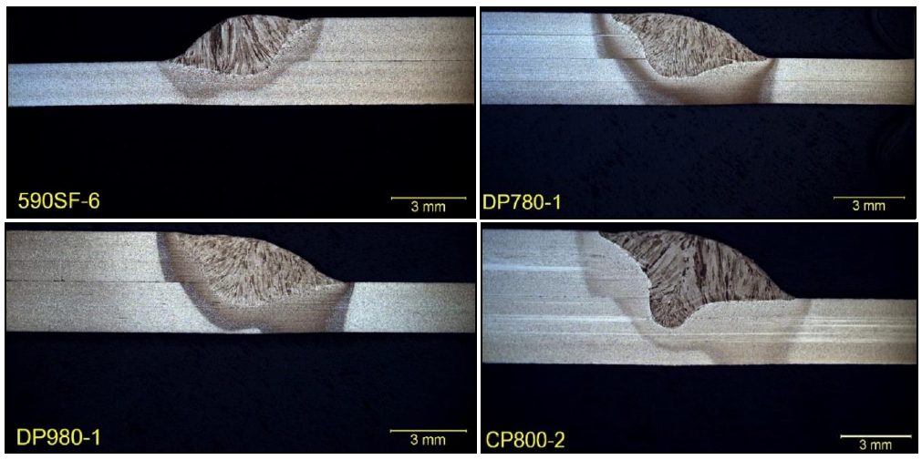
Figure 4: Cross Sections of Lap Joints (etched with 2% Nital).M-13
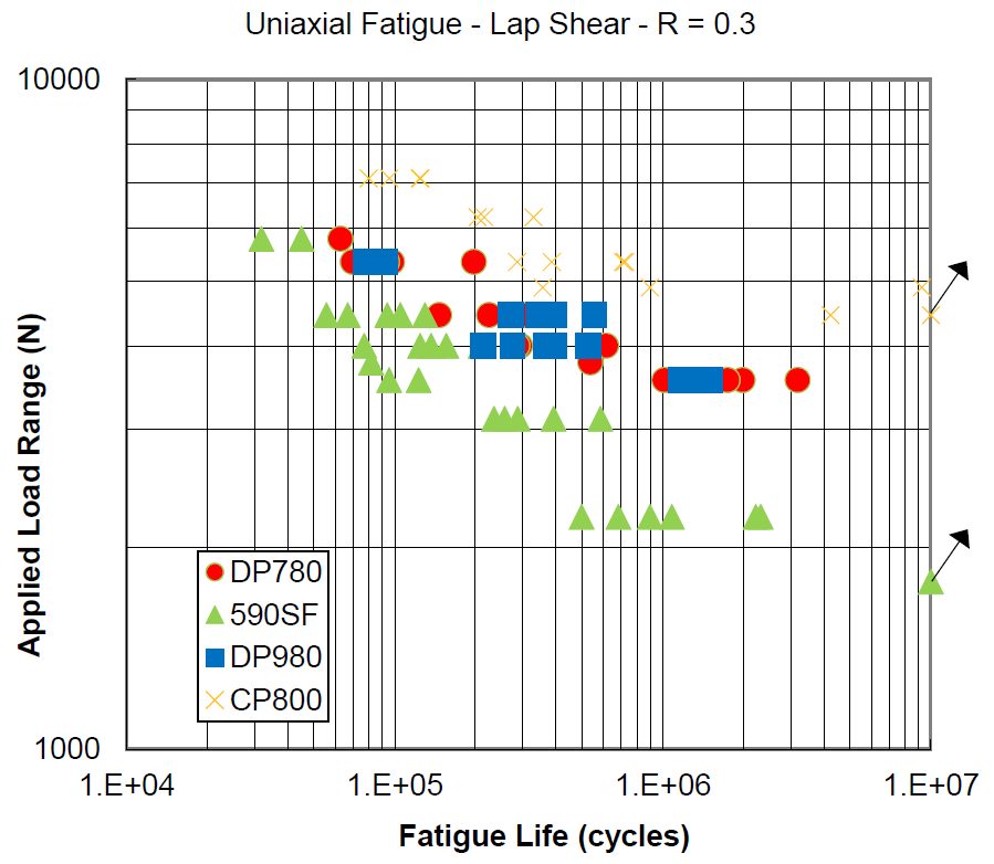
Figure 5: Results of Fatigue Testing in Tension at R= 0.3.M-13
Weld root cracking dominated in the 590 SF, as well as the DP 780 and DP 980, with an example shown in Figure 6. Weld toe cracking was observed on the 2.8-mm-thick CP 800, with an example shown in Figure 7.
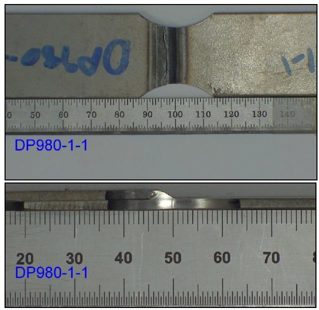
Figure 6: Example for a Root Crack Breaking Through the Weld Metal on DP 980.M-13
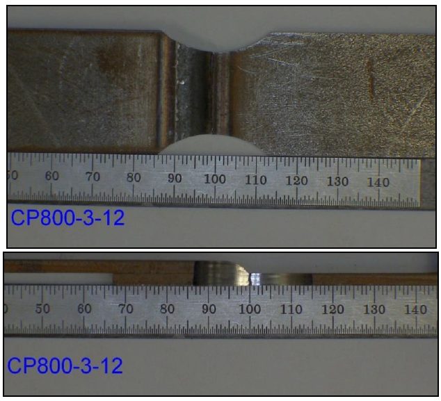
Figure 7: Example of a Toe Crack Breaking Through the Base Metal.M-13
Fatigue testing in bending at R = -1 gave lifetimes between 30,000 and 2 million cycles, with run-outs on tests that continued to up to 7 million cycles, as shown in Figure 8.
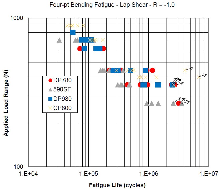
Figure 8: Four-Point Bending Tests at R = -1.M-13
Taking the differing thicknesses, minor variations in minimum width, and the stress concentrations from the radii into account, the concentrated stress range was calculated to compare the four materials on a common basis, as shown in Figure 9.
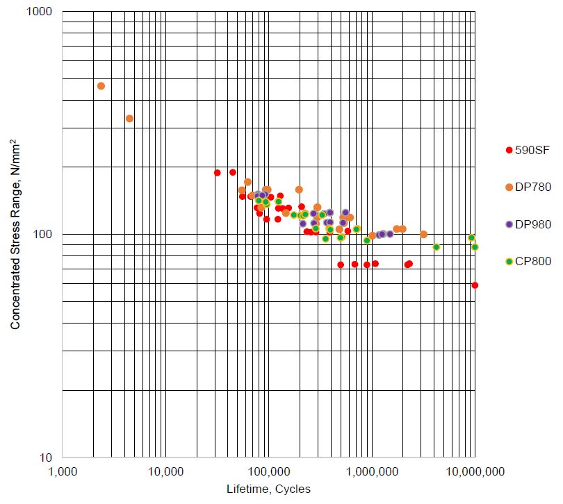
Figure 9: Concentrated Stress Range versus Lifetime for Tension Tests.M-13
The fatigue cracks initiated at the root for the 1.8-mm 590 SF on both tension and bending testing. The fatigue cracks initiated at the weld toe for the 2.8-mm CP 800 on both tension and bending testing. The fatigue cracks initiated from the weld root in the tension testing and from primarily the weld cap in bending testing, for the 2.0-mm-thick DP 780 and 2.0-mm-thick DP 980.
This articles summarizes a paper entitled, “New Test to Analyze Hydrogen Induced Cracking Susceptibility in Resistance Spot Welds,” by M. Duffey.D-10
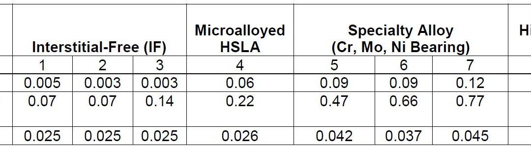
This study aims to develop a new weldability test to analyze the susceptibility of HIC in RSW of different steels. A total of eight different steel samples were analyzed with their carbon content, associated American Welding Society (AWS) carbon equivalencies, and gauges shown in Table 1. All materials were tested in the full-hard condition (all have been cold-rolled).
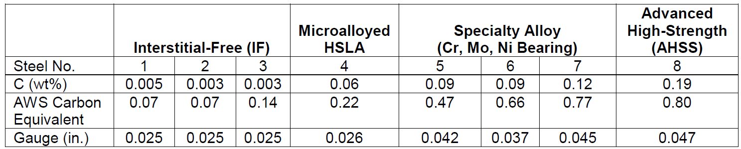
Table 1: Tested Steels, Carbon Equivalencies, and Steel Gauge.D-10
The associated parameter ranges for welds made with each steel are in Table 2. The resistance spot weld was made in the middle of the sheets, as shown in the test setup in Figure 1. There was a total of 18 test samples (nine not painted and wiped, nine painted) for each material tested.

Table 2: Welding Parameters.D-10
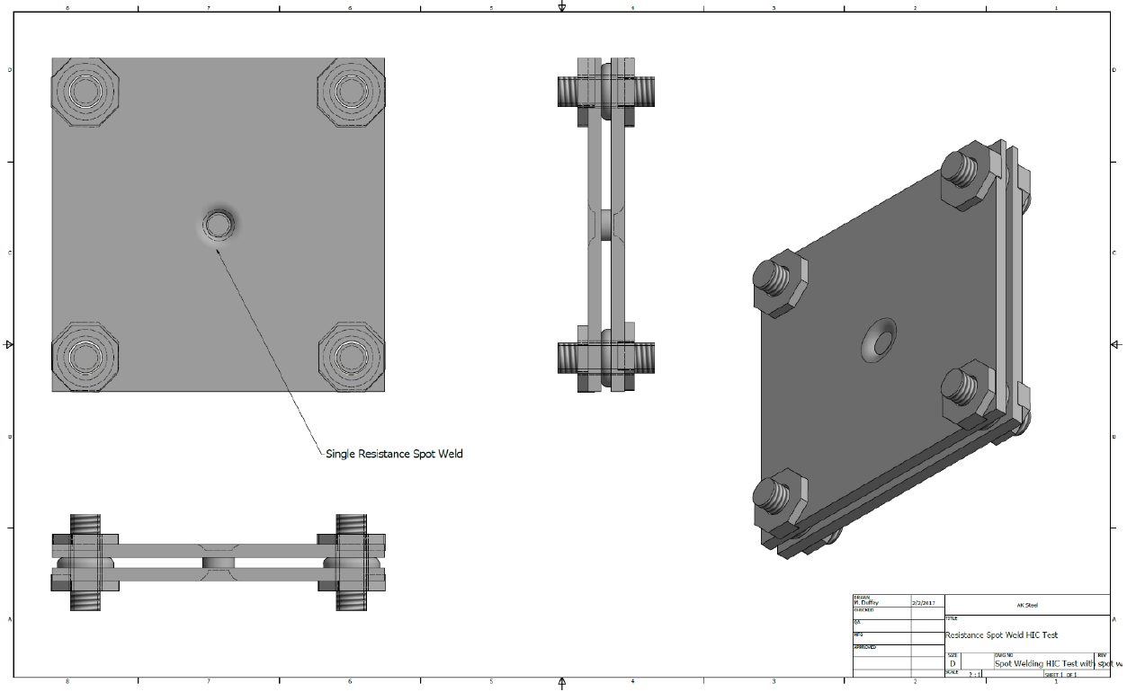
Figure 1: HIC Test for Resistance Spot Welds Schematic.D-10
Figure 2A shows the results of the 3- × 3-in. tests. Figure 2B shows the results of the 4- × 4-in. tests. Figure 2C shows the results of the 5- × 5-in. tests.
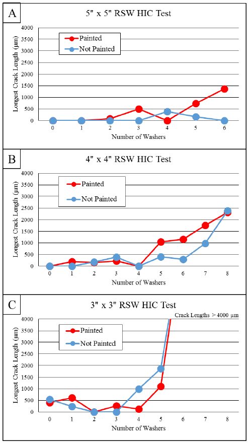
Figure 2: Results of the Three Different Test Sizes on AHSS.D-10
Cracks consistently initiated at the periphery of the weld nugget where the two steel sheets came together. Cracks then propagated either in the weld metal or HAZ, as shown in Figures 3 and 4.
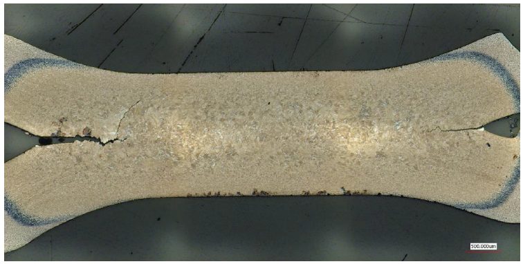
Figure 3: Cracking in the Weld Metal of Steel 8.D-10
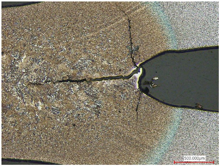
Figure 4: Cracking in Both the Weld Nugget and HAZ in Steel 8.D-10
Figure 5 displays the results from Steels 1, 4, and 5. Steel 1 is the most resistant (of the three) to HIC. For the three steels shown in Figure 5, the crack length (at each gap spacing) was longer for the painted sample than the non-painted sample.
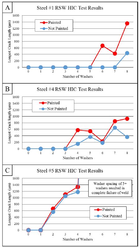
Figure 5. Test Results for Steels 1, 4, and 5.D-10
The microstructure of IF Steels 1-3 (Figure 6A) was ferrite. The microstructure of the high-strength low-alloy (HSLA) Steel 4 (Figure 6B) was a mixture of grain boundary ferrite, martensite, and possibly some bainite. The microstructure of the specialty alloy Steels 5-7 and AHSS Steel 8 (Figure 6C) was entirely martensite.
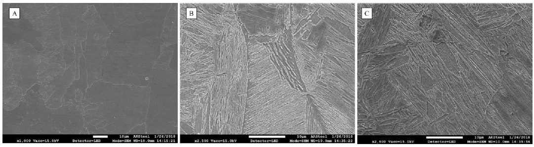
Figure 6: Microstructures of the Different Weld Nuggets.D-10
Figure 7 shows the fracture surface of a crack completely through Steel 7.
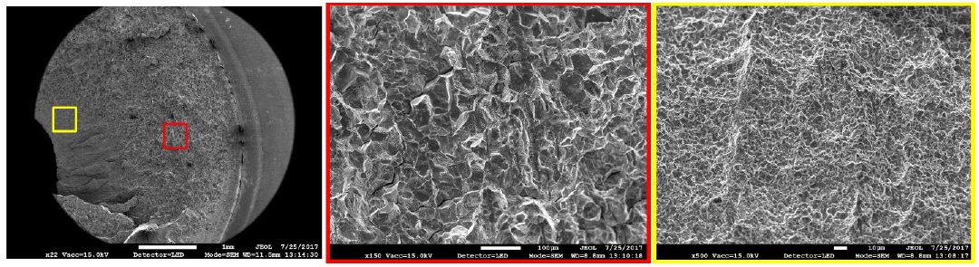
Figure 7: Fracture Surface of Cracked Weld in Steel 7.D-10
The average and maximum hardness results of spot welds in each material are summarized in Figure 8.
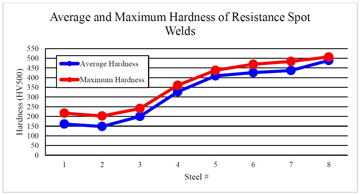
Figure 8. The Average and Maximum Hardness of HAZ and Weld Nugget in Resistance Spot Welds of Each Steel.D-10
Figure 9 is a graph that displays the carbon equivalence, number of washers where cracking first began, and average hardness of the weld nugget and HAZ in each steel.
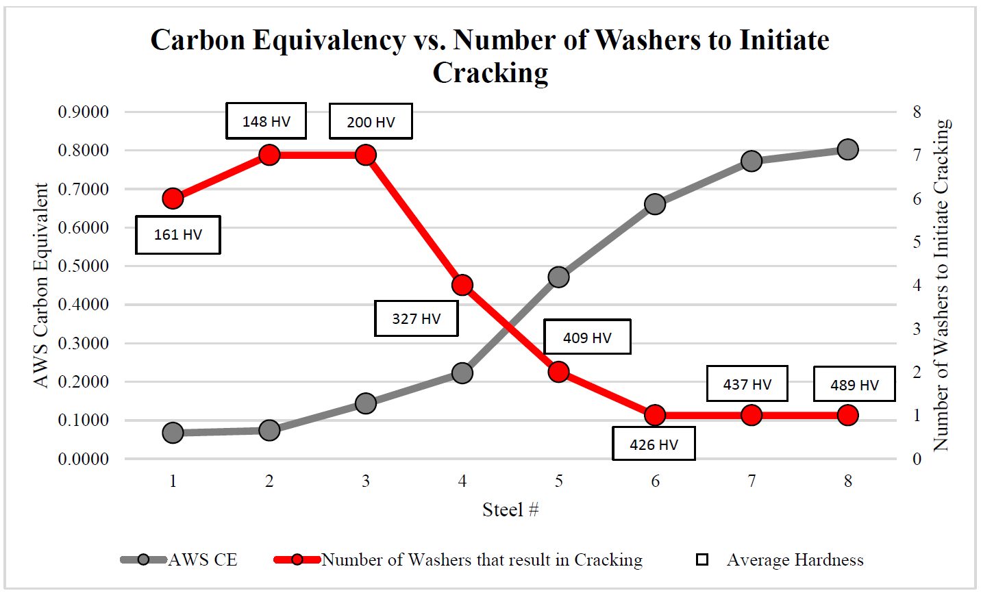
Figure 9: Carbon Equivalency vs. Number of Washers to Initiate Cracking.D-10
M-12. A. Mohamadizadeh, E. Biro, N. Zhou, and M. Worswick, “3D Processing Maps and Constitutive Modeling of Spot Welds in Hot-Stamping Automotive Steels,” Sheet Metal Welding Conference XVIII Livonia, MI October 17-18, 2018.